Portable & Mobile Monopoles · Volume 1
The Portable-Monopole Problem
Counterpoise without a ground system, and the physics of loading — the handheld body-counterpoise problem and the tiger tail, the Chu/Wheeler/Harrington small-antenna limit stated precisely, and why loading position (base vs. center vs. top) governs every shortened portable whip's efficiency
1.1 About this volume
The fixed-vertical-monopoles dive built its entire foundation on one clean idealization: a quarter-wave conductor over a ground plane good enough to approximate the perfect-conductor image theory gives you, refined by a buried or elevated radial field engineered specifically to hold that approximation together. That idealization is not available here. A portable or mobile monopole — a handheld’s stub whip, a vehicle-mounted mobile antenna, a backpack HF vertical unrolled on a summit — has no permanent radial field, no buried copper, and usually no say in the matter at all: the “ground” it gets is whatever conductive or lossy structure happens to be nearby when the PTT button goes down. Sometimes that structure is genuinely good (a vehicle’s steel roof at VHF/UHF, which spans several wavelengths and behaves close to an infinite sheet). Sometimes it is the operator’s own body, a lossy, high-permittivity, constantly-moving dielectric mass that was never designed to be part of an antenna. Sometimes, if the operator skips the counterpoise wire that came in the box, it is nothing at all, and the antenna radiates against whatever capacitive coupling to earth it can scavenge.
This volume owns the physics that decision imposes, in the abstract, before the catalogue of specific hardware gets built out. Two structurally different problems recur across every portable and mobile antenna this dive covers, both consequences of the missing engineered ground. The first is the counterpoise problem: what does the antenna’s return current actually flow through, and how does that choice change with grip, posture, and deployment discipline? §3 works this through for the handheld case, the starkest version of the problem and the one every ham has felt directly. The second is the small-size problem: HF wavelengths are tens of meters, a backpack or a vehicle roof is not, and every portable HF antenna in this hub’s later volumes is built on some form of physical shortening plus reactive loading to compensate. §4 states precisely what the Chu/Wheeler/Harrington limit does and does not forbid about small antennas — a distinction routinely garbled in ham forum folklore — and §§5–7 develop the loading physics (current distribution, coil Q, radiation-resistance collapse, and the efficiency relation) governing every base-, center-, and top-loaded portable whip the rest of this dive describes. §8 closes with a single reconciled efficiency-by-band table, replacing the two overlapping tables this dive’s earlier migrated content carried.
What this volume deliberately does not do is catalogue hardware. There is no ham-stick bill of materials here, no MP-1 spec sheet, no commercial-buy ranking. Those belong to Vol 2 (vehicle-mobile mounts, the roof-as-ground-plane physics, and the VHF/UHF whip catalogue — which sets up, but does not solve, the mobile-HF problem), Vol 3 (ham-sticks, resonators, and screwdriver mobile HF whips; the backpack-portable HF survey — MP-1, AX-1, Buddistick, Wolf River Coil; and the counterpoise-deployment discipline that makes or breaks all of it), and Vol 4 (VHF/UHF deploy-and-go, rubber ducks and aftermarket whips, and SDR-receive telescoping whips), with Vol 5 carrying the DIY build, the commercial-buy survey, and the companion gear and gotchas. Every number those volumes quote for a specific antenna’s efficiency, bandwidth, or loading scheme is an instance of the physics this volume derives; get the physics right once, here, and the per-product numbers downstream become legible rather than memorized.
1.2 Why a portable monopole is a structurally different antenna
A fixed vertical and a portable vertical can be, in the limit, geometrically identical pieces of aluminum tubing — the same quarter-wave (or shortened-and-loaded) conductor, the same 36 Ω image-theory feedpoint target, the same standing-wave current and voltage distribution the fixed-vertical dive’s Vol 1 derives from the method of images. What separates the two families is not the radiator; it is what stands in for the other half of the image-theory picture — the return path the base current has to complete before it gets back to the transmitter. Fixed-vertical Vol 1 §6 introduced loss resistance R_loss as the series term that real, imperfect ground stacks on top of the idealized 36 Ω radiation resistance, and the entire companion Vol 2 of that dive is a treatise on driving R_loss down with an engineered radial field — sixty-plus buried radials, or a handful of elevated ones, purpose-built and permanently installed specifically to approximate the perfect-conductor image plane the theory assumes.
A portable installation cannot make that investment, and the consequence is that the identity of the counterpoise — not just its quality, but what physical structure is playing that role at all — becomes a first-order design variable rather than an engineered constant. Four distinct regimes recur across this dive, worth naming up front because Vols 2–4 each live almost entirely inside one of them. A vehicle roof at VHF/UHF is the closest a portable installation gets to the fixed-vertical ideal: at 446 MHz a typical sedan roof spans on the order of two wavelengths per side, close enough to an infinite conducting sheet that a roof-center NMO whip performs comparably to a well-grounded fixed vertical. A vehicle roof at HF, by contrast, is electrically minuscule — a 20 m mobile installation’s “ground plane” is a few percent of a wavelength across, closer to a point than a plane — and works mainly through resistive/capacitive coupling of the vehicle body to earth rather than anything resembling the image-theory idealization; Vol 2 covers why this makes mobile HF structurally harder than mobile VHF/UHF even before §5’s loading question stacks on top. The operator’s own body, developed in full in §3, is the counterpoise for every handheld transmission, whether the operator thinks about it or not. And a deliberately deployed counterpoise wire or wire set — the tiger tail on a handheld, the four 12-ft radials fanned from an MP-1’s base — is the one case where the operator engineers the return path directly, on a scale of minutes rather than a permanent installation, which is exactly why Vol 3 treats deploying it correctly as mandatory rather than optional.
The through-line across all four regimes is that the antenna’s radiating geometry and its return-path geometry are being solved as two separate, often badly mismatched problems, in a way a fixed vertical’s designer never confronts because the radial field is specified, installed, and left alone. A portable operator re-solves the counterpoise problem every time they change grip, walk to a different spot on a summit, or forget to unroll a wire — and every efficiency number this dive’s later volumes quote for a specific antenna is conditional on which counterpoise regime that measurement assumed. This volume’s job is to make that conditionality explicit rather than an unstated asterisk on every spec sheet.
1.3 The handheld counterpoise problem — body current, grip, and the tiger tail
Every quarter-wave (or loaded, electrically-shortened) whip needs a return path for the RF current that flows out the base as the same current flows up the radiator. On a base-fed fixed vertical that return path is the radial field; on a handheld transceiver there is no radial field, and the radio’s own PCB ground and battery pack are far too small, electrically, to serve as an adequate counterpoise on their own at HF or low VHF. What completes the circuit instead is whatever conductive, lossy structure is physically closest to the radio: the operator’s hand gripping the case, the forearm, and — coupled more weakly through intervening tissue and clothing — the rest of the torso. Skin-effect current flows on the surface of all of it, at RF, the moment the PTT key closes, whether the operator is aware of the mechanism or not.
This is why a handheld’s measured performance is so sensitive to details that have nothing to do with the whip itself. Grip changes the antenna. A hand wrapped around the radio’s lower body couples differently to the whip’s near field than a hand holding the radio by a belt clip or lanyard, and the difference shows up as a real shift in feedpoint impedance and radiated field strength — the “antenna,” electrically, includes the hand, and moving the hand moves the antenna. Setting the radio down disconnects the counterpoise almost entirely. A handheld resting on a wooden table or a car dashboard loses the operator’s body from the circuit and is left radiating against whatever residual capacitive coupling the radio’s own chassis and battery pack offer the surrounding room — commonly reported in ham field practice as a noticeable signal drop, on the rough order of several decibels, though the precise figure depends heavily on the radio, the surface, and the band, and no single number should be treated as a rigorous laboratory result rather than a widely repeated field observation.
The direction of the body-proximity effect specifically is worth stating more carefully than ham folklore usually does, because two competing mechanisms are at work and they do not always point the same way. Holding the radio close to the chest adds real conductive and capacitive mass to the counterpoise side of the circuit, which is the mechanism that improves the return path relative to holding the radio away from the body with a minimal grip. But human tissue is also a lossy, high-water-content dielectric that absorbs RF directly, and at the higher end of the UHF amateur range in particular, near-field power dissipated in nearby tissue is a real loss mechanism competing against the counterpoise-improvement effect — which is also part of why RF-exposure evaluations for handhelds specifically model the body as a lossy load rather than a benign conductor. Which mechanism dominates for a given radio, band, and body position is not something this volume can responsibly reduce to a single directional rule, and the honest statement is that the net effect is band- and geometry-dependent, and field reports in the ham community are correspondingly mixed — some operators find performance improves against the chest, others find no change or a slight degradation, and a rigorous side-by-side measurement isolating the two competing mechanisms for a specific handheld is the only way to settle it for that radio.
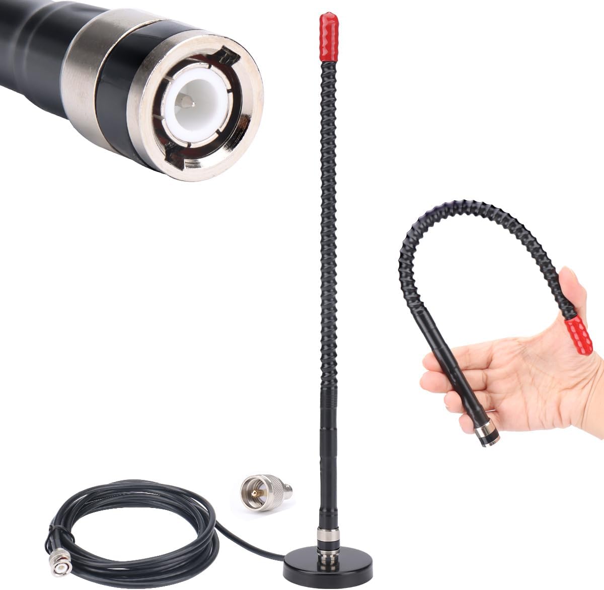
What is not ambiguous is the value of giving the antenna a deliberate, engineered counterpoise instead of relying on whatever the operator’s incidental body position happens to provide. The “tiger tail” is exactly that: a length of wire, cut to a quarter-wavelength at the operating frequency, with one end clamped at the antenna’s ground reference (the BNC or SMA shell, or the case’s ground point) and the other end left free, hanging loose from the radio. Electrically it is a deliberately deployed counterpoise wire in miniature — the same idea §2 named as the fourth counterpoise regime, just scaled down to fit in a shirt pocket. The length follows directly from the same quarter-wave constant the fixed-vertical dive derives for a physical monopole element — L_feet ≈ 234/f_MHz for thin wire — because a counterpoise wire lying against or near the operator’s body is, electromagnetically, playing the same current-carrying role a physical radial does, just unbalanced and close-coupled rather than laid out flat on open ground. At the 2 m calling frequency used elsewhere in this hub’s length tables (146.00 MHz), that formula gives 234/146.00 ≈ 1.60 ft ≈ 48.9 cm — close to the roughly 19-inch figure commonly quoted in ham tiger-tail how-to material, the small difference being ordinary cut-and-trim tolerance rather than a contradiction. At 446.00 MHz the same formula gives 234/446.00 ≈ 0.52 ft ≈ 16.0 cm, again close to (if a centimeter or so shorter than) the roughly 16.5 cm figure that circulates in some published tiger-tail instructions — a gap well within the tolerance any builder should expect to trim out with an antenna analyzer rather than treat as a fixed dimension.
Mechanistically, the tiger tail works by giving the near-field return current a defined, low-loss conductor instead of forcing it entirely through the variable, lossy geometry of hand-and-body coupling — it supplements the body as a counterpoise with something the return current prefers, closer to resonant length and cleaner than tissue and clothing. The improvement is real and repeatedly reported, but this volume will not manufacture a false-precision decibel figure for it: field reports commonly cite low-single-digit-decibel gains on both transmit and receive, with the honest caveat that rigorously controlled A/B measurements isolating the tiger tail’s own contribution from grip and posture variance are scarce — the right reading for a specific radio and band is “a genuine, small, worthwhile improvement,” not a number to build a link budget on.
1.4 The small-antenna limit — Chu, Wheeler, Harrington, and ka
Every shortened portable antenna this dive covers — a base-loaded ham-stick on 80 m, a center-loaded MP-1 on 40 m, even a helically-wound rubber duck on 2 m — is an electrically small radiator by the standard definition, and the theory that bounds what a small antenna can and cannot do was worked out well before any of that specific hardware existed. H. A. Wheeler, in “Fundamental Limitations of Small Antennas” (Proceedings of the IRE, vol. 35, Dec. 1947, pp. 1479–1484), introduced the governing size parameter: with k = 2π/λ the free-space wavenumber and a the radius of the smallest sphere that encloses the radiating structure, the dimensionless product ka measures electrical size independent of frequency or physical scale. Wheeler’s key observation was that a sphere of radius a = 1/k (i.e., ka = 1) marks a meaningful physical boundary — inside it, an electrically small antenna’s near field is dominated by reactive, non-propagating stored energy rather than by the radiating far field, a region the later small-antenna literature commonly calls the radiansphere. An antenna with ka < 1 lives mostly inside that boundary: most of the energy sloshing in its near field never leaves as radiation on a single cycle, and that stored reactive energy relative to the radiated energy is exactly what determines how sharply tuned — how high-Q — the structure has to be.
L. J. Chu, in “Physical Limitations of Omni-Directional Antennas” (Journal of Applied Physics, vol. 19, no. 12, Dec. 1948, pp. 1163–1175), turned Wheeler’s qualitative picture into a quantitative bound. Modeling the field outside the enclosing sphere as an expansion in spherical vector wave modes and asking what the minimum possible Q is for an antenna confined to that sphere and radiating through its lowest-order mode, Chu derived the widely quoted result
Q_min = 1/(ka)³ + 1/(ka),
a bound that applies to any lossless antenna — of any internal geometry whatsoever — confined within a sphere of radius a. For ka well below 1 the 1/(ka)³ term dominates completely, and Q rises explosively as the antenna is packed into an ever-smaller fraction of a wavelength: halving ka roughly octuples the minimum achievable Q. R. F. Harrington, in “Effect of Antenna Size on Gain, Bandwidth, and Efficiency” (Journal of Research of the National Bureau of Standards, Section D: Radio Propagation, vol. 64D, no. 1, Jan.–Feb. 1960, pp. 1–12), generalized Chu’s single-mode treatment to antennas that use multiple spherical modes simultaneously, tightening the bound in the multi-mode case and connecting it explicitly to achievable gain as well as Q — the combined result is what the antenna literature has come to call the Chu–Harrington limit, and it is the fundamental ceiling every electrically small antenna in this dive operates under.
It is worth being precise about what that ceiling does, because the ham-forum shorthand — “small antennas are inefficient, it’s a law of physics” — mangles the actual claim in a way that matters for how you read every efficiency table downstream. The Chu–Harrington limit bounds Q — and through Q, fractional bandwidth — for a given electrical size. It does not, by itself, bound efficiency. A lossless, perfectly conducting antenna built to the smallest possible ka can, in principle, radiate essentially all of the power delivered to it — high efficiency and small size are not in direct conflict. What the limit does force is that such an antenna will necessarily be extraordinarily high-Q, and Q sets bandwidth by the familiar approximate relation fractional bandwidth ≈ 1/Q (a first-order approximation; the exact relationship between Q and a given VSWR-defined bandwidth carries a further, VSWR-dependent constant that this volume will not derive, but 1/Q is the right order-of-magnitude statement for the point being made here). A small, efficient antenna is therefore a small, narrowband antenna — sharply tuned, unforgiving of frequency drift, and typically needing a matching network re-tuned by hand or by servo motor every time the operating frequency moves by more than a fraction of a percent. The alternative — the move every practical shortened HF portable actually makes — is to deliberately trade efficiency for bandwidth: adding real loss resistance (a lower-Q loading coil, a lossy matching network, a resistive broadbanding element) lowers the achieved Q well below Chu’s lossless floor, which widens the usable bandwidth exactly as intended, at the direct cost of dissipating more of the input power as heat instead of radiation. Both outcomes are fully compliant with the Chu–Harrington bound; the bound is silent on which one a given design chooses, because efficiency is governed by a separate, ordinary circuit relation — the loss-resistance argument of §7 — layered on top of the fundamental size/Q relationship, not derived from it.
Grounding this in the portable-monopole scale makes the abstraction concrete. Take a generic 2 m physical whip section — the rough scale of a ham-stick’s fiberglass mast, independent of any specific commercial product — operated first on 80 m (design frequency 3.650 MHz, λ ≈ 82.19 m) and then on 40 m (7.150 MHz, λ ≈ 41.96 m). On 80 m, h/λ ≈ 0.0243, so ka = 2π(h/λ) ≈ 0.153, and Chu’s formula gives Q_min ≈ 1/(0.153)³ + 1/0.153 ≈ 286 — an enormous minimum Q, implying a lossless-limit fractional bandwidth under half a percent, on the order of 10–15 kHz at 3.65 MHz. On 40 m the same whip sits at h/λ ≈ 0.0477, ka ≈ 0.300, Q_min ≈ 41 — dramatically lower and more forgiving to tune. A 3 m whip on 20 m (14.175 MHz, λ ≈ 21.16 m, h/λ ≈ 0.142, ka ≈ 0.89) sits close to the ka = 1 radiansphere boundary, Q_min ≈ 2.5 — hardly constrained by Chu’s bound at all, which is exactly why 20 m portable whips can be built both broadband and efficient in a way an 80 m ham-stick fundamentally cannot. This ordering — 80 m brutally high-Q, 40 m moderate, 20 m nearly unconstrained — matches the well-known field experience that low-band mobile/portable HF antennas are notoriously fussy to keep on frequency while upper-HF portable whips tune broadly: the Chu–Harrington relationship showing up as lived operating experience. §8’s real-world efficiency figures for these bands fall well short of what Chu’s lossless Q ceiling implies, because §6’s loading-coil losses have already broadbanded these antennas at an efficiency cost the fundamental limit never required in the first place.
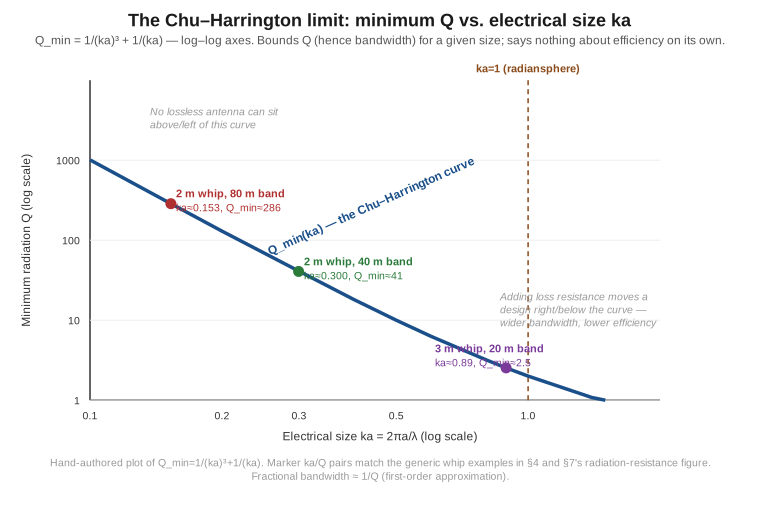
Q_min = 1/(ka)³ + 1/(ka), and three illustrative portable-whip points on it. The curve bounds achievable bandwidth for a given size; it says nothing about efficiency on its own — a design can sit on the curve (narrowband, low-loss) or move to the right of it by adding loss resistance (broader, less efficient), but it cannot move left of the curve at a given ka.1.5 The physics of loading — base, center, and top
A physical quarter-wave conductor is, at HF, routinely longer than any portable installation can carry: 234/f_MHz gives roughly 20.5 m on 80 m and 10.5 m on 40 m, both hopeless for a backpack or a vehicle mount. Every portable HF antenna this dive covers responds to that mismatch the same way: shorten the physical conductor, and add series reactance somewhere along it to cancel the capacitive reactance the shortening introduces, restoring an electrically resonant (or near-resonant) feedpoint on a physically manageable structure. That added reactance is almost always inductive — a wound coil — because canceling capacitive reactance without adding physical length requires an inductor, and the coil’s placement along the shortened element, not merely its value, turns out to be the single most consequential design decision in the whole antenna.
The reason placement matters follows directly from the current distribution the fixed-vertical dive’s Vol 1 derives for a full-size element: current maximum at the driven base, falling to zero at the open tip, following the standing-wave cos(βz) envelope. Cut the conductor short of a full quarter-wave and drive it as an open-circuited transmission-line stub, and the exact current distribution becomes I(z) = I₀ · sin(β(h−z))/sin(βh) for a physical height h measured from the base — which, in the electrically-short limit βh ≪ 1, collapses to the simple triangular approximation I(z) ≈ I₀ · (h−z)/h: current falling linearly from the base value to zero at the tip, rather than following the gentler cosine curve a full-size element enjoys. That triangular taper is the unloaded (or purely base-loaded) short monopole’s natural current distribution, and it is the worst-performing shape available, because the effective average current over the physical structure — what actually matters for radiation — is only half the base value.
Where the loading coil sits changes this picture directly, because the coil itself carries no radiating current worth speaking of (it is a lumped, non-radiating component regardless of where it sits) while the wire on either side of it carries whatever current distribution the boundary conditions leave it. Base loading places the coil right at the feedpoint, between the transmitter and the entire physical radiator: the whole exposed conductor is now “above the coil,” and it inherits the triangular taper described above stretched across its full — if short — physical length, exactly the worst case above. Center loading moves the coil partway up the structure, typically near or above its geometric midpoint: the section of wire below the coil, from the base up to the coil, is short enough electrically that it carries close to the full base current with only a modest taper, while only the shorter section above the coil — from the coil to the tip — suffers the triangular falloff to zero. Moving the coil up trades a full-height taper for a partial one, and because only the smaller above-coil section pays the penalty, the antenna’s effective height rises substantially relative to the base-loaded case, even though the coil’s electrical value and the antenna’s total physical height have not changed at all. Top (capacitive-hat) loading goes further still: instead of a series inductor anywhere along the wire, a shunt capacitive structure at the physical tip — described fully in §6 — sustains the current close to its base value essentially all the way to the top, because the hat’s capacitance to free space does the reactance-canceling job an inductor would do elsewhere, but does it at the open end rather than partway down. The current profile that results is close to flat over the antenna’s whole physical run — the same “uniformly high current over the full structure” profile a genuinely taller radiator would show — which is exactly why top loading is, current-distribution-wise, the best of the three.
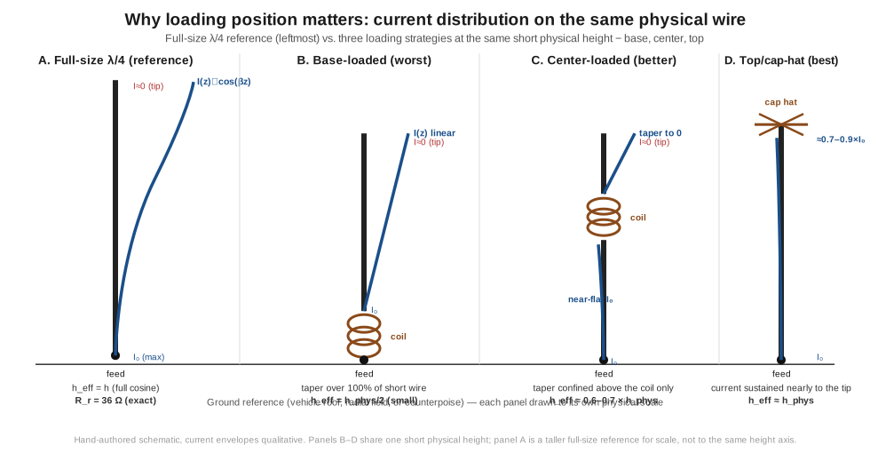
The ranking — top loading best, center loading next, base loading worst — is not a rule of thumb invented for portable gear; it is the same conclusion the fixed-vertical dive’s Vol 4 reaches for shortened fixed verticals, worked there against a broadcast-scale 160 m example. What genuinely differs at portable scale is the mechanical option set: a fixed vertical bolted to a permanent mast can carry a wire-spoke capacitive hat a meter or more across, because it never has to collapse into a backpack or a vehicle trunk. A ham-stick, an MP-1, a Wolf River Coil, a Buddistick — every backpack- or trunk-mounted portable HF antenna Vol 3 catalogues — is built around a coil, not a hat, precisely because an effective capacitive hat’s mechanical footprint is incompatible with the collapsibility the whole product category exists to provide. Ham-sticks are base-loaded by design (the coil sits where the antenna screws onto the mobile mount); the MP-1, Wolf River Coil, and Buddistick family are center-loaded, the coil positioned partway up the mast and often tap-adjustable to retune across bands. This is a real, structural handicap the portable category carries relative to its fixed-vertical cousin: portable HF antennas are, almost without exception, stuck at the base- or center-loaded end of the ranking above, not because their designers chose poorly, but because the mechanical constraint that defines “portable” rules out the one loading position that performs best.
1.6 Coil Q, loss resistance, and capacity hats
The loading coil that restores resonance to a shortened whip is not a lossless component, and how lossy it is matters as much as where it sits. A real inductor’s quality factor is defined the ordinary way, Q = X_L/R_coil, where X_L is the coil’s reactance at the operating frequency and R_coil is the equivalent series resistance — winding-wire ohmic loss, proximity- and skin-effect loss between adjacent turns, and, for a coil wound on a magnetic core rather than air, core loss — dissipating real power as heat instead of passing it to the radiating structure above. A well-wound, air-core loading coil at HF, of the scale used in ham-stick and MP-1-class antennas, is commonly reported in the loaded-vertical literature to reach a Q on the order of 100–300; the exact figure depends on wire gauge, winding pitch, coil diameter, and, for a switched or tapped multi-band design, the resistance the tap contact itself adds in series. A physically larger coil, wound with heavier wire on a larger-diameter form, generally achieves a higher Q than a compact coil squeezed into a collapsible whip section, for the same reason a bigger conductor always beats a smaller one on ohmic loss — part of why a “bugcatcher”-style coil, unconstrained by a slim telescoping tube, is commonly reported to outperform a compact motor-driven screwdriver coil of the same electrical value.
The loss resistance the coil contributes is R_coil = X_L/Q, and because a heavily shortened whip needs a large inductance to cancel its correspondingly large capacitive reactance, X_L itself can be substantial even before dividing by Q — exactly why the coil’s contribution to total loss resistance, not just its Q in isolation, is what a builder needs to track. §7 puts a number on how this stacks up against the antenna’s already-tiny radiation resistance; the point to carry here is that a heavily-shortened portable’s loading coil is very often the single largest loss term in the system, larger than any residual ground- or body-coupling loss, because the coil’s job (cancel a large reactance) and its loss mechanism (dissipate power proportional to that reactance divided by a finite Q) are two sides of the same component.
Capacitive top hats — the technique §5 identified as the best-performing loading position — work by an entirely different mechanism than a coil, and are worth understanding on their own terms even though, as that section noted, they are mechanically rare on truly collapsible portable gear. A hat is a small horizontal (or slightly domed) structure of wire spokes or a wire cage mounted at the physical top of the shortened radiator and bonded to it electrically; its capacitance to the surrounding free space cancels the element’s residual capacitive reactance at the open end rather than partway down the wire, which is what lets the current stay close to its base value all the way to the physical tip instead of tapering away. The rule that follows is unambiguous: a larger hat is a better hat, because more capacitance holds more current further out along the physical structure, pushing the effective height closer to the true physical height. This is precisely why the technique dominates at fixed installations — a broadcast tower’s wire-and-guy umbrella, or an amateur fixed vertical’s spoke-and-radial hat, can be built as large as the mast can structurally support — and why it is nearly absent from the true backpack-portable category: an MP-1 or Buddistick occasionally uses a short flared tip or a small end-loading element that captures a fraction of the hat effect, but the capacitance achievable from anything that has to collapse into a tube small enough to fit in a pack is a small fraction of what even a modest fixed-installation hat provides, and no portable design in this hub’s catalogue relies on top-hat loading as its primary mechanism the way a Marconi-T fixed vertical does.
1.7 Radiation-resistance collapse and the efficiency relation
The current-distribution argument of §5 has a precise quantitative form, and it is the same relation the fixed-vertical dive’s Vol 4 derives for shortened fixed verticals: for a short monopole, radiation resistance follows the small-antenna relation
R_r ≈ 160π² · (h_eff/λ)² Ω,
where h_eff is the effective height — the current-weighted average of the actual distribution over the physical structure, normalized to the base current — rather than the physical height itself. h_eff equals the true physical height only in the idealized uniform-current (perfect top-hat) case; for the triangular taper of an unloaded or base-loaded short monopole, h_eff = h_physical/2, and because the relation is quadratic, halving the effective height does not halve R_r, it quarters it. This is worth working through with a concrete, generic example rather than leaving it abstract: take the same 2 m physical whip used in §4’s illustration, operated on 80 m (λ ≈ 82.19 m). In the idealized best case — uniform current over the full 2 m, as a large, well-built top hat would approximate (h_eff = h = 2 m, h_eff/λ ≈ 0.0243) — the formula gives R_r ≈ 1579 × (0.0243)² ≈ 0.93 Ω. In the base-loaded, triangular-taper case (h_eff = 1 m, h_eff/λ ≈ 0.0122), the same formula gives R_r ≈ 1579 × (0.0122)² ≈ 0.23 Ω — a factor of roughly four lower, exactly the quadratic penalty the halved effective height predicts, and broadly consistent in order of magnitude with the fixed-vertical dive’s own worked numerical example for a comparably small ka (a roughly 10°-tall 160 m radiator there, reported at 0.3 Ω triangular-taper vs. 0.97 Ω top-loaded — the same physics, a different band and physical scale, landing in the same numerical neighborhood). On 40 m (λ ≈ 41.96 m), the identical 2 m whip’s uniform-current ceiling rises to R_r ≈ 1579 × (2/41.96)² ≈ 3.59 Ω, and its triangular-taper floor to R_r ≈ 0.90 Ω — both roughly quadrupled relative to 80 m, because the whip is now a larger fraction of the (shorter) wavelength. It bears repeating, per the caveat the sibling dive also flags, that this h² relation is a small-antenna approximation, accurate while h_eff/λ stays well under roughly 0.1–0.15; it should not be extrapolated all the way out to a genuine λ/4, where the true cosine-distribution result — the fixed-vertical dive’s own derived 36 Ω — governs instead, and the two curves are deliberately not merged into one continuous line in the figure below.
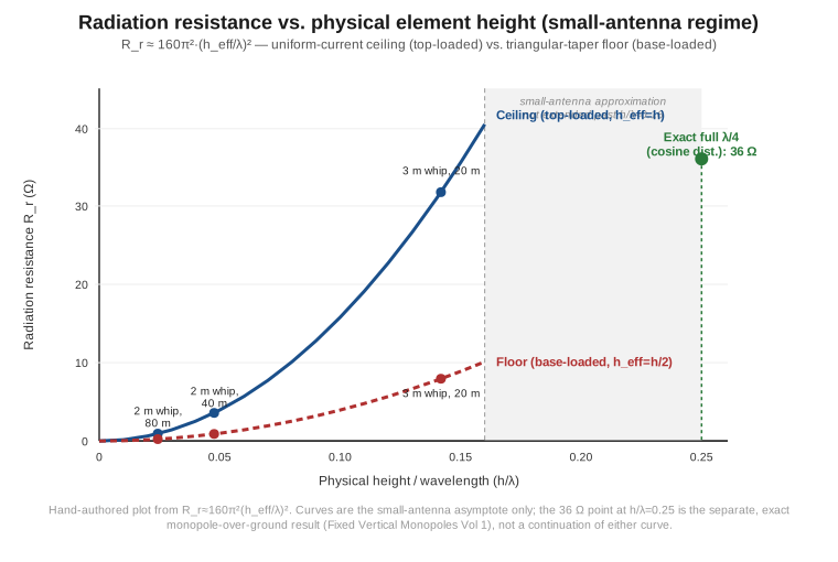
h_eff = h, top-loaded) and the triangular-taper floor (h_eff = h/2, base-loaded). Three illustrative generic-whip points are marked; the curve is drawn only over the small-antenna regime where the h² approximation holds. At h/λ = 0.25 the true (cosine-distribution) full-size monopole resistance is the fixed-vertical dive's derived 36 Ω — off this approximation entirely, and marked separately rather than as a continuation of either curve.Radiation resistance by itself does not determine how much of the transmitter’s power leaves as radio waves; that is the job of the efficiency relation the fixed-vertical dive’s Vol 1 establishes and this dive inherits unmodified:
η = R_rad / (R_rad + R_loss),
with R_loss now standing for whatever series loss resistance the installation’s counterpoise regime and loading hardware contribute — §6’s coil loss plus whatever residual body- or ground-coupling loss §§2–3 described, all lumped into one series term. The arithmetic is unforgiving because R_rad has already collapsed to a fraction of an ohm on the low bands: the 80 m base-loaded example above (R_rad ≈ 0.23 Ω) has to be paired with a loss resistance that is honestly derived rather than assumed, and the derivation is unforgiving. A 2 m whip on 80 m presents a capacitive reactance of roughly −2300 Ω, so the loading coil must supply about +2300 Ω to reach resonance, and §6’s R_coil = X_L/Q then sets the floor: even an excellent air-core coil at Q ≈ 300 contributes R_coil ≈ 7.6 Ω, while the compact, densely-wound coil a real ham-stick actually carries (Q ≈ 100–150) contributes 15–23 Ω. Add vehicle-body and ground-return loss on top and R_loss lands in the 15–35 Ω range, giving η ≈ 0.7–1.5%. It is worth pausing on what that arithmetic rules out: an R_loss of 2 Ω on this antenna — a figure that looks innocuous and gets quoted casually — would require a coil Q of over 1100, which no practical loading coil approaches. 80 m mobile is a one-percent-efficiency proposition, not a ten-percent one, and any source quoting the latter has skipped this step. On 40 m, R_rad ≈ 0.90 Ω against the same 15–35 Ω loss budget (the required X_L halves, but so does little else) gives η in the 2.5–5.6% range; on 20 m, where the whip is barely shortened (h/λ ≈ 0.14, the uniform-current ceiling near 32 Ω) and the loading coil is correspondingly small or absent, a modest R_loss of 5–10 Ω gives η in the 75–85% range. That last figure deserves an explicit caveat rather than a confident quotation: at h/λ ≈ 0.14 the whip sits at the very edge of the small-antenna window this section just declared, so the 32 Ω ceiling is an optimistic upper bound rather than a tight estimate, and the 75–85% efficiency that follows from it should be read the same way — the right order of magnitude, and the right qualitative conclusion (20 m portable operation is genuinely efficient in a way 80 m never is), but not a number to design against. This progression — brutal on 80 m, workable on 40 m, comfortable on 20 m — is exactly §8’s table, falling directly out of the same R_rad ∝ h_eff² then η = R_rad/(R_rad+R_loss) machinery applied at three electrical sizes.
1.8 Efficiency by band — a reconciled table
The table below consolidates the band-by-band efficiency picture this dive’s earlier migrated content had spread across two overlapping tables — one keyed to a general “practical portable antenna” boundary, the other specific to ham-stick mobile whips — into a single reference, grounded in the R_rad/η arithmetic of §7 and the design frequencies this hub’s other volumes already use for band-length tables. Where a range is wide, the spread reflects loading position as much as band: a base-loaded ham-stick and a center-loaded MP-1-style antenna on the same band, at similar physical height, land at different points within the same row, exactly the §5 ranking predicts. These figures are representative and order-of-magnitude, not a guarantee for any specific product — Vols 2–3 give the per-antenna numbers where a manufacturer’s own or independently measured data exists.
That form-factor column is doing real work and deserves to be named rather than left as an implicit detail: this table does not hold one physical antenna fixed across all nine rows. It follows the band-appropriate form factor a sensible portable operator would actually reach for — a ~2 m loaded whip on 80 and 40 m, where nothing shorter is practical and nothing longer is portable; a ~3 m lightly-loaded whip on 20 m, where the size penalty starts to ease; a full-size telescoping whip from 17 m up, where one is mechanically practical at all. That distinction is what governs how this table relates to the companion one in Vol 3 §3, which holds a single fixed ~7 ft base-loaded ham-stick across every band instead. On 80 and 40 m the two tables describe the same hardware and therefore agree — a ~2 m loaded whip is what both assume, and both land on the one-to-low-single-digit-percent figures §7’s loss-budget derivation forces. From 30 m upward they part company, and the reason is entirely the form factor: this table lets the antenna grow and shed its loading coil as the wavelength shortens, while the ham-stick stays one physical design, so its figures run progressively lower — widest around 20 m, then narrowing toward 12/10 m as the fixed stick’s own height finally closes in on a comparable fraction of λ/4. Both are honestly derived from the same physics; the gap above 30 m is the fixed-hardware penalty a ham-stick pays for covering ten bands with one design, not a disagreement to average away.
Table 1 — 8. Efficiency by band — a reconciled table
| Band (design freq) | Free-space λ | Typical portable form factor | h/λ (illustrative) | Loading | Typical efficiency |
|---|---|---|---|---|---|
| 80 m (3.650 MHz) | 82.2 m | ~2 m loaded whip (ham-stick / mobile HF class) | ~0.024 | base to center | 1–2% |
| 40 m (7.150 MHz) | 42.0 m | ~2 m loaded whip | ~0.048 | base to center | 3–6% |
| 30 m (10.125 MHz) | 29.6 m | ~2–2.5 m loaded whip | ~0.07–0.08 | center | 18–30% |
| 20 m (14.175 MHz) | 21.2 m | ~3 m whip, lightly loaded/near full-size | ~0.14 | minimal | 55–80% |
| 17/15 m (18.118 / 21.225 MHz) | ~16.6 / 14.1 m | full-size or near-full-size telescoping whip | ~0.18–0.24 | none to minimal | 65–85% |
| 12/10 m (24.940 / 28.500 MHz) | ~12.0 / 10.5 m | full-size fiberglass or telescoping whip | ~0.25+ | none | 75–90% |
| 6 m (50.250 MHz) | 5.97 m | full-size whip | ~0.25 | none | 85–95% |
| 2 m (146.00 MHz) | 2.05 m | full-size whip + counterpoise | ~0.25 | none | 90%+ (helical stub: 5–15%) |
| 70 cm (446.00 MHz) | 0.673 m | full-size whip + counterpoise | ~0.25 | none | 90%+ (helical stub: 5–15%) |
The “helical stub” parenthetical on the 2 m and 70 cm rows is a deliberate flag rather than an afterthought: a rubber-duck-style helically-wound handheld antenna is not a straight shortened monopole in the sense §5–7 analyze, and its radiation resistance does not follow the same simple h_eff/λ scaling this section’s arithmetic used — the helix winds the conductor into a compact form whose electromagnetic behavior is genuinely its own topic (normal-mode helix theory), not a straightforward loading-position variant of the whip physics this volume develops. Vol 4 treats rubber ducks and their aftermarket full-size replacements on their own terms; the 5–15% figure quoted here is the well-established real-world efficiency range reported for stock helical stubs, carried forward for table completeness, not derived from this section’s monopole formula.
1.9 Where this volume hands off
This volume established the physics that governs every portable and mobile monopole this dive will catalogue. §2 framed the structural difference from the fixed-vertical case: the counterpoise is not an engineered constant but a variable the operator re-solves every time grip, posture, deployment, or vehicle changes. §3 worked the handheld case through — body current as an incidental, variable counterpoise, and the genuine, honestly-hedged benefit of a deliberately deployed tiger tail sized by the same 234/f_MHz constant the rest of this hub uses. §4 stated the Chu–Harrington limit precisely — a bound on Q and therefore bandwidth for a given electrical size, not a direct bound on efficiency, with the real efficiency story following instead from the separate loss-resistance argument §§5–7 developed: the loading-position ranking (top best, center next, base worst), the R_r ≈ 160π²(h_eff/λ)² relation and its quadratic sensitivity to effective height, the coil-Q loss mechanism dominating a heavily-shortened portable’s loss budget, and the η = R_rad/(R_rad+R_loss) relation tying it all together into the §8 reconciled table.
Everything from here is the application of this physics to specific hardware. Vol 2 covers vehicle-mobile installations — mag-mount and NMO VHF/UHF whips riding the good-ground-plane regime §2 named, and the roof-as-ground-plane physics that sets up, without solving, the mobile-HF problem. Vol 3 covers mobile and portable HF proper — ham-stick and screwdriver mobile whips living squarely in this volume’s base-to-center loading-position analysis, plus the backpack-portable family (the MP-1, AX-1, Buddistick, and Wolf River Coil), center-loaded almost without exception for the mechanical reasons §5 gave, and the counterpoise-wire deployment discipline that determines whether a given unit reaches §8’s efficiency figures or instead operates against the operator’s body and the soil underfoot at a fraction of that number. Vol 4 covers VHF/UHF deploy-and-go antennas (J-pole and Slim Jim), rubber ducks and their full-size aftermarket replacements — where §8’s helical-antenna caveat gets its full treatment — and telescoping whips for SDR receive, where relaxed receive-only constraints make much of this volume’s efficiency arithmetic close to irrelevant. Vol 5 closes the dive with a DIY build, the ranked commercial-buy survey, companion gear, and the gotchas and myths — including the “high-gain rubber duck” claims this volume’s physics already rules out — recurring across the whole portable-and-mobile family.
1.10 Resources
- H. A. Wheeler, “Fundamental Limitations of Small Antennas,” Proceedings of the IRE, vol. 35, Dec. 1947, pp. 1479–1484 — the radiansphere concept and the
kasize parameter this volume’s §4 builds on. - L. J. Chu, “Physical Limitations of Omni-Directional Antennas,” Journal of Applied Physics, vol. 19, no. 12, Dec. 1948, pp. 1163–1175 — the minimum-Q bound
Q_min = 1/(ka)³ + 1/(ka)for an antenna confined to an enclosing sphere. - R. F. Harrington, “Effect of Antenna Size on Gain, Bandwidth, and Efficiency,” Journal of Research of the National Bureau of Standards, Section D: Radio Propagation, vol. 64D, no. 1, Jan.–Feb. 1960, pp. 1–12 — the multi-mode generalization of Chu’s bound, and the combined result the literature calls the Chu–Harrington limit.
- Balanis, Antenna Theory: Analysis and Design (4th ed.) — the short-dipole/monopole radiation-resistance derivation (
R_r ∝ (h_eff/λ)²) this volume’s §7 builds on, shared with the sibling Fixed Vertical Monopoles Vol 4. - W8JI (Tom Rauch), “Short Verticals” and “Mobile Antennas, Short Verticals, Loading Coil Loss, and Loading Coil Current” (w8ji.com) — the loading-position current-distribution argument and worked efficiency examples this volume’s §5–7 draw on, developed in full for the fixed-vertical case in the sibling dive.
- ARRL Antenna Book (25th+ ed.) — the vertical-antenna and mobile/portable chapters underlying the loading-position ranking and the general shortened-antenna guidance this volume reconciles at portable scale.
- The fixed-vertical-monopoles dive — the image-plane theory, 36 Ω/5.15 dBi reference figures, and engineered-radial-field treatment this volume’s §2 contrasts against.
- The single-band-dipoles dive — the standing-wave current/voltage picture and cut-to-length arithmetic this whole hub’s monopole family, portable included, inherits.
Comments (0)