Fixed Vertical Monopoles · Volume 2
Pattern, Ground Effect & the Radial Field
The low-angle elevation lobe over perfect vs real ground and the pseudo-Brewster degradation, the omnidirectional azimuth circle, the radial system as the antenna's other half — quantified efficiency from bare ground to sixty buried radials to four elevated ones — and why ground loss widens (and lies about) the SWR curve
2.1 About this volume
Vol 1 fixed the quarter-wave monopole’s geometry and its feedpoint: the image-plane derivation that makes a grounded λ/4 element electrically half of a half-wave dipole, the resulting ≈36 Ω resonant feedpoint (36 + j0 Ω once trimmed, half the dipole’s 73 Ω), the standing-wave current and voltage distributions on the element, and the introductory statement of the radial system’s job — replacing lossy real earth with a low-resistance return path for the near-field current. That volume owns the feedpoint; this one owns everything the feedpoint’s output actually does once it leaves the wire; where the power goes in angle, and how much of it survives the trip through the ground system on the way there.
Those two questions are inseparable for a vertical in a way they are not for a dipole, and that is the whole reason this volume exists as the dive’s center of gravity. A dipole’s pattern and a dipole’s efficiency are nearly independent facts — a full-size copper dipole radiates at very close to 100% efficiency regardless of how you feed it, and the interesting pattern story is purely a matter of height above ground. A vertical’s pattern and efficiency are the same fact wearing two hats. The radial field is not a footnote to the antenna; it is the other conductor of a two-conductor radiating structure, and how well it does its job simultaneously sets how much power leaves the system at all (efficiency) and, in the practical case, distorts where that power goes once it does (the real-ground pattern degradation this volume quantifies in §3). Get the radial system wrong and you do not get a slightly-worse version of the textbook vertical; you get a fundamentally different antenna — an inefficient, high-angle noise magnet wearing the shape of a DX performer.
This volume’s lane is therefore three things, taken in order. First, the radiation pattern — the textbook perfect-ground elevation lobe Vol 1 already quoted at 5.15 dBi, developed here into where in elevation that gain actually sits, and how thoroughly real, lossy ground disturbs the answer (§2–3), plus the omnidirectional azimuth pattern and its real-world caveats (§4). Second, and the section this dive is built around, the radial field’s efficiency — the formal η = R_rad/(R_rad + R_loss) relationship, quantified from a bare-ground vertical’s 3–10 dB of heat loss through a serious 60-radial buried field’s 0.5–1 dB down to a 4-radial elevated counterpoise’s sub-0.3-dB figure, and why those numbers land where they do (§5–8). Third, the SWR and bandwidth behaviour, and the specific trap that ground loss sets for anyone reading a SWR meter as a proxy for antenna quality (§9). What this volume does not do is repeat Vol 1’s feedpoint derivation, matching-network survey, or the standing-wave picture — those are cited, not rebuilt — and it does not carry the full-size trap-vertical product survey, the shortened/loaded-vertical efficiency penalty, or the hands-on build and radial-installation procedure, which belong to the volumes that follow this one in the dive. Every pattern figure here is a model-derived canonical shape (NEC or method-of-moments over the stated ground model), and the prose flags explicitly where a real installation will differ from the idealization.
2.2 The low-angle advantage over perfect ground
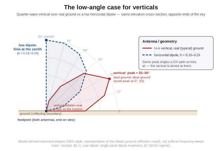
Start from the number Vol 1 already quoted and take it one derivation further: a quarter-wave monopole over a perfect, infinite conducting ground plane radiates, in the upper half-space, exactly the upper half of a half-wave dipole’s donut — the same cos((π/2)cos θ)/sin θ pattern factor, with θ measured from the vertical element itself, restricted to 0° ≤ θ ≤ 90°. The critical difference from a horizontal dipole over ground is that the monopole’s own feedpoint sits at the ground reference (height zero relative to its own image), so there is no height-dependent interference term splitting the pattern into lobes the way the horizontal-dipole pattern-and-ground treatment develops for a dipole raised above a separate ground plane. There is one lobe, and reading the pattern factor at its own natural boundary — θ = 90°, straight out along the ground — gives cos(0)/sin(90°) = 1: the maximum. Over a perfect ground, a quarter-wave vertical’s peak gain of 5.15 dBi sits exactly at the horizon, 0° elevation — not lifted to some compromise angle by height, because there is no height to speak of. The pattern falls off smoothly from that peak as θ decreases from 90° (elevation rises from 0°), reaching the same end-on null at θ = 0° (straight up, the zenith) that a dipole shows off its own tips — the donut’s hole, pointed at the sky.
This is worth sitting with, because it is a stronger and cleaner claim than “verticals are good for DX,” and it is the theoretical ceiling every real installation is measured against. Zero-degree elevation is as low as an elevation angle can physically go; a genuine DX path arriving at 3–8° over the true horizon is a path a perfect-ground vertical would serve better than one arriving at 20°, because the perfect-ground pattern is still climbing toward its peak as elevation falls toward zero. A horizontal dipole cannot make this claim at any height: the single-band-dipole pattern-and-ground treatment shows every horizontal-dipole elevation lobe has a hard null exactly at the horizon, a consequence of the 180° phase reversal a horizontally-polarized wave suffers on ground reflection. The vertical’s ground reflection for vertically-polarized fields does not carry that same forced reversal — over a perfect conductor the vertically-polarized reflection coefficient is +1 at every angle, constructively reinforcing the direct wave all the way down to grazing incidence rather than cancelling it there. That single polarity difference in the boundary condition is the entire reason a vertical, and not a low dipole, is the textbook low-angle DX antenna, and it is worth naming explicitly rather than waving at “verticals are omnidirectional and low-angle” as received wisdom.
None of this happens over real ground, and that gap between the clean theoretical peak and what actually radiates off your quarter-wave whip is the subject of the next section — but it is essential to have the perfect-ground answer nailed down first, because the real-ground story is entirely a story about how far short of “gain still climbing at zero elevation” reality falls.
2.3 Real ground and the pseudo-Brewster degradation
Real soil is a lossy dielectric, not a perfect conductor, and the vertically-polarized reflection coefficient off a lossy boundary is not the flat +1 of §2 at every angle. The Fresnel reflection coefficient for a wave whose E-field lies in the plane of incidence — which is the geometry of a vertically-polarized wave reflecting off the ground beneath a monopole — is
Γ_∥(Δ) = [ε_c sin Δ − √(ε_c − cos²Δ)] / [ε_c sin Δ + √(ε_c − cos²Δ)],
where Δ is the elevation (grazing) angle measured up from the horizon and ε_c = ε_r − j·60λσ is the ground’s complex relative permittivity (ε_r the ordinary dielectric constant, σ the conductivity in S/m, λ in metres). For a lossless dielectric (σ = 0, ε_c real), this expression passes exactly through zero at the true Brewster angle — total transmission, no reflection, at one specific angle. Real soil is never lossless, so Γ_∥ never reaches zero; instead its magnitude dips to a shallow minimum and its phase swings rapidly through roughly 90° over a narrow angular window near that same angle — the pseudo-Brewster angle. Crucially, that dip sits at grazing angles that are small but not zero for ordinary soil, and the reflection coefficient’s magnitude at true grazing incidence (Δ → 0) is markedly below the perfect-conductor’s +1, with a phase that is no longer a clean 0°. The consequence for the elevation pattern is immediate: the coherent, constructive, in-phase addition that pinned the perfect-ground peak at Δ = 0° in §2 no longer happens at Δ = 0° over real ground — the field at true grazing is genuinely weaker (this is the same physics, at longer range, that makes AM broadcast ground-wave signal strength fall off with distance even over reasonably conductive soil), and the pattern’s actual maximum is pushed up off the horizon to whatever angle balances “still fairly low” against “past the worst of the pseudo-Brewster dip.”
Where that balance lands depends on soil conductivity, and the direction of the dependence is the one every vertical-antenna discussion eventually gets to: better (more conductive) soil pushes the peak closer to the ideal 0°, and worse soil pushes it further up and knocks more gain off the top. The table below reproduces the standard NEC/method-of-moments result for a resonant quarter-wave vertical over homogeneous ground of the stated conductivity, referenced against the perfect-ground ceiling from §2. The figures are representative of the low HF bands (modeled around 7 MHz over a competent ~60-radial system, following the Cebik/Michaels ARRL data); both the peak angle and the peak gain shift with frequency and with the radial system, so read them as order-of-magnitude, not spec-sheet, values:
Table 1 — Where that balance lands depends on soil conductivity, and the direction of the dependence is the one every vertical-antenna discussion eventually gets to: better (more conductive) soil pushes the peak closer to the ideal 0°, and worse soil pushes it further up and knocks more gain off the top. The table below reproduces the standard NEC/method-of-moments result for a resonant quarter-wave vertical over homogeneous ground of the stated conductivity, referenced against the perfect-ground ceiling from §2. The figures are representative of the low HF bands (modeled around 7 MHz over a competent ~60-radial system, following the Cebik/Michaels ARRL data); both the peak angle and the peak gain shift with frequency and with the radial system, so read them as order-of-magnitude, not spec-sheet, values
| Ground quality | Conductivity (S/m, approx.) | Peak elevation angle | Peak gain | Delta from the 5.15 dBi / 0° ideal |
|---|---|---|---|---|
| Perfect ground (image theory) | ∞ | 0° (at the horizon) | 5.15 dBi | — reference |
| Salt water | ~5 | ~0–3° | ~4.5–5.15 dBi | near-ideal — peak stays near the horizon, gain nearly preserved |
| Wet, fertile farmland | ~0.03 | ~15–21° | ~1.5–2 dBi | ~3–3.5 dB down |
| Typical / average soil | ~0.005 | ~20–27° | ~0–0.5 dBi | ~4.5–5 dB down |
| Dry, rocky, or sandy soil | ~0.001 or less | ~25–35°+ | ~−2 to 0 dBi | ~5–7+ dB down |
Two things are worth pulling out of that table. First, salt water is the one soil good enough to approximate the perfect-ground assumption, which is the entire reason beachfront and island DXpeditions post such outsized signal reports on 40, 80, and 160 m from unremarkable-looking verticals — the pseudo-Brewster degradation genuinely nearly vanishes over seawater, and the textbook 5.15 dBi is close to what actually radiates. Second, the elevation-angle shift is not a cosmetic detail — a vertical over typical soil is putting its peak lobe at 20–27° rather than 0°, which is a perfectly serviceable DX angle but is not the near-grazing angle the perfect-ground picture promises, and a vertical over genuinely poor (dry, rocky, sandy) soil pushes that peak high enough, and knocks enough gain off it, that the low-angle advantage over a modest horizontal dipole starts to erode. This is the honest answer to “why does my vertical seem to underperform the spec sheet” for an installation on poor ground: the antenna is not broken, and it is not undersized — it is doing exactly what a resonant quarter-wave element over that particular soil’s Fresnel reflection coefficient is capable of doing, and the radial system (§5 onward) only fixes the near-field return-current loss, not this far-field reflection-coefficient degradation. A better radial field cannot buy back the pseudo-Brewster loss; only better native soil, or moving the reflecting surface (elevating the whole system, or choosing a wetter site), can do that. The two loss mechanisms are genuinely separate, and conflating them is a common source of frustration when a textbook-radial installation still under-performs its site’s inherent ground quality.
2.4 Azimuth — the omnidirectional circle
The azimuth story is mercifully simpler than the elevation one, because the vertical element and a competently symmetric radial field are both rotationally symmetric about the vertical axis, and neither the pattern factor of §2 nor the ground-reflection physics of §3 depends on azimuth at all. The theoretical azimuth pattern is therefore a perfect circle — equal gain in every compass direction — which is the vertical’s other headline advantage over a dipole: no orientation decision, no favoured broadside direction, no end-on nulls to steer around.
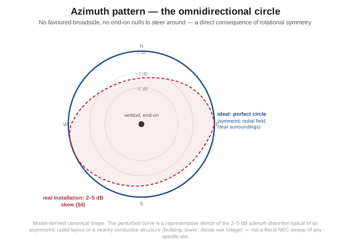
That symmetry is a property of the idealized installation, not a law of physics that survives contact with a residential lot. Two things break it in practice, and both trace back to the radial field rather than the whip. An asymmetric radial layout — radials bunched into the only quadrant of the yard that has room, or a fence or slab forcing half the field shorter than the other half — breaks the rotational symmetry the pattern factor assumes and skews the azimuth response toward the side with the more complete ground system, typically by a couple of dB rather than a dramatic reshaping. Nearby conductive structures — a metal roof, a second tower, a chain-link fence, even a stand of wet trees — act as passive parasitic reflectors and re-radiators, adding constructive gain on the side they sit and subtracting it on the opposite side; a rule of thumb worth carrying is at least a wavelength of genuinely clear space in the azimuth direction that matters most, which on 40 m is 40 m of clearance and is often the binding constraint on a residential lot rather than the vertical’s own footprint. Neither effect changes the elevation story of §2–3; they perturb the azimuth circle into an ellipse-with-bumps typically within 2–5 dB of the ideal, which is a real and worth-knowing number but a second-order correction next to the radial-field efficiency question that dominates the rest of this volume.
2.5 The radial field as the other half of the antenna
Vol 1 introduced the radial field’s job in a sentence: replace lossy real earth with a low-resistance artificial conductor for the near-field return current. This section makes that sentence quantitative, because the quantity is what separates a vertical that works from one that doesn’t.
The governing relationship is ordinary circuit-level radiation efficiency, and it is worth writing out in full because every number in the rest of this volume is a restatement of it. The vertical’s radiation resistance — the R_rad ≈ 36 Ω Vol 1 derived from the image-plane theory — is a fixed property of the element’s geometry; it does not change with how good or bad your ground system is. What the ground system controls is a series loss resistance, R_loss, that appears in series with R_rad at the feedpoint and represents every ohm of resistive, non-radiating dissipation the return current encounters on its way from the base of the radial field back to the feedpoint — soil resistance heating, contact resistance at joints, and (for buried systems) dielectric loss in the near-surface earth. The fraction of input power that actually leaves as radiation, the radiation efficiency, is simply
η = R_rad / (R_rad + R_loss),
and the corresponding loss in decibels is 10·log₁₀(η) (a negative number, conventionally quoted as its magnitude — “3 dB of loss” means η = 0.5). This is precisely the same efficiency bookkeeping that governs a shortened, loaded element’s coil losses or a lossy matching network — a series resistance that does not radiate divides the input power between “radiated” and “heat” in exact proportion to how it compares with the radiating resistance it sits beside. For a vertical, R_rad is small (36 Ω, versus a dipole’s 73 Ω), which is exactly why the radial field matters so much more here than a BALUN’s core loss matters for a dipole: the same handful of ohms of R_loss is a much larger fraction of a 36 Ω total than it would be of a 73 Ω one.
Running that formula against the headline figures this dive has been building toward makes the point concrete. A vertical with no radial system, or a token few thrown down as an afterthought, loses 3–10 dB — an efficiency of roughly 50% down to 10%, which back-solves through the formula above to an effective R_loss running from about 35 Ω at the mild end to well over 300 Ω at the severe end; that is genuinely “most of your transmitter’s power is heating the dirt under the antenna,” not a rounding error. A serious buried radial field — on the order of 60 quarter-wave radials over typical soil — brings the loss down to 0.5–1 dB, an efficiency of 79–89%, corresponding to an R_loss of roughly 4–9 Ω. And a mere four elevated, resonant radials do better still — under 0.3 dB, over 93% efficient, R_loss under about 2.6 Ω. Those R_loss figures are not independently measured constants pulled from a datasheet; they are the algebra of η = R_rad/(R_rad + R_loss) run backward from the dB figures that the antenna-modeling and field-measurement literature (Brown, Lewis & Epstein’s 1937 broadcast-ground-system study and the later NEC-based confirmations discussed in §6–7) converges on. Presenting them this way is deliberate: it turns “0.5 dB, sounds fine” into “a few ohms of loss resistance sitting in series with a 36 Ω radiator,” which is the frame an EE reads much faster than a decibel does, and it is also the frame that makes the diminishing-returns curve of the next section make sense as a resistance problem rather than a mystery percentage.
2.6 Buried radials — the diminishing-returns curve
The radial-count-versus-efficiency relationship for a buried ground system is one of the oldest quantitative results in antenna engineering — it dates to George Brown, Robert Lewis and Joseph Epstein’s 1937 Bell Labs / RCA study of AM broadcast ground systems, and it has been reproduced and refined by every ground-system modeling effort since, from the ARRL Antenna Book’s own tables through to the modern NEC-based work most visibly associated in the amateur literature with Rudy Severns, N6LF. The shape of the result — not the exact figure at any one radial count, which shifts with soil and frequency, but the shape — is consistent everywhere it has been checked, and it is the shape a builder needs internalized: efficiency rises quickly with the first several radials and then flattens hard, so that doubling a large radial count buys far less than doubling a small one did.
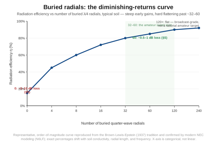
The physical reason the curve bends over rather than continuing to improve linearly is a parallel-resistance argument any EE will recognize instantly. Model each buried radial as presenting some effective series resistance to the portion of the near-field return current it intercepts; N such radials, if they behaved as fully independent parallel paths, would combine to a total ground resistance that falls roughly as 1/N — the classic “resistors in parallel” scaling, and it is exactly why the first handful of radials buy the largest gains (going from 1 parallel path to 2 halves the resistance; going from 60 to 120 barely moves it). But buried radials laid at realistic azimuthal spacing are not independent: adjacent radials at a few degrees of separation share much of the same near-field soil volume and couple to each other, so the effective parallel-path count saturates well below the literal radial count once spacing drops below roughly the soil’s effective “coupling radius.” That coupling is precisely why the curve flattens rather than tracking 1/N all the way to arbitrarily small resistance, and it is why radial length interacts with radial count — a sparser field of longer radials intercepts return current over a wider area with less mutual coupling than a denser field of the same total wire crowded into a smaller radius, so a design with fewer, longer radials can outperform a naive count-only comparison.
Reading the curve for a design decision: the steep early region — zero to roughly a dozen or two buried radials — is where a builder gets the most return on labor, typically covering the gap from the pathological 3–10 dB region of §5 down into the 1–2 dB range. Pushing on to the 32–60-radial range that §5 quoted (0.5–1 dB) is a genuinely serious commitment of wire and trenching, and it is the point most amateur installations reasonably stop, because the next doubling — 60 to 120, the historical AM-broadcast “full” ground system — buys only a few more tenths of a dB. Beyond about 120 radials the curve is essentially flat; broadcast engineering pushes there because a few tenths of a dB matters commercially at the coverage-contour level for a station with no atmospheric noise floor to hide behind, but it is not a rational target for an amateur station where atmospheric and receiver noise floors swamp a 0.2 dB difference in transmitted power. The practical amateur answer the curve encodes is the same one Vol 1 already gestured at: somewhere in the 32–60-radial range is the sweet spot where the labor curve and the efficiency curve cross in the builder’s favor, with anything beyond that best spent on other parts of the station.
2.7 Elevated radials — the counterpoise that beats more buried wire
The elevated-radial result — that as few as four resonant, elevated counterpoise wires can out-perform tens of buried ones — reads as a contradiction of the parallel-resistance logic in §6 until the mechanism is made explicit, and the mechanism is worth stating plainly: an elevated radial’s return current flows through air, not through lossy earth, so it simply does not accumulate the ground-resistance term the buried case is fighting in the first place. A buried radial field is fundamentally a damage-control structure — it exists to intercept current that would otherwise flow through the surrounding soil and dissipate there, and no matter how many parallel paths you add, you are still routing current through a lossy medium and hoping the low-resistance wire captures most of it before the soil does. An elevated system sidesteps the problem instead of mitigating it: raised clear of the ground (typically a fraction of a wavelength — high enough that the near-field coupling back down into the earth beneath the radials is small) and cut to resonant quarter-wave length, four symmetric elevated wires establish the antenna’s counterpoise reference almost entirely through a near-lossless conductor, because there is no lossy dielectric in the current’s path to speak of.
That is also why the radial count requirement collapses from dozens to single digits. The buried case needs many radials because each one is a lossy, partial solution to an earth-conduction problem and more of them in parallel is the only lever available. The elevated case needs only enough radials to establish rotational symmetry and a well-defined, resonant counterpoise structure — a job that a single radial does badly (badly asymmetric, no useful counterpoise reference, on the order of 30–50% efficiency by itself), two opposite radials do adequately (75–85%), and four arranged with 90° rotational symmetry do essentially completely (90–95%, matching the sub-0.3-dB figure §5 quoted), with six or eight buying only marginal further improvement. Four is not an arbitrary round number here; it is the smallest radial count that gives the structure genuine rotational symmetry in two orthogonal axes, and that symmetry — not sheer wire count — is what an elevated system is actually selling.
The price of that efficiency is that an elevated system trades the buried field’s forgiving, largely non-resonant construction for a genuinely tuned structure. A buried radial does not need to be cut to any particular electrical length to do its job — it is a bulk conductor draining current out of the near-field zone, and burying it in reasonably conductive earth damps out any resonant behavior it might otherwise show, which is why buried-radial practice tolerates radials shorter than a full quarter-wave (at a modest, quantifiable efficiency penalty) and does not fuss over cutting each one to an identical, precise length. An elevated radial, floating in low-loss air, behaves like exactly what it is — a quarter-wave resonant element — and each one has to be cut close to resonance and matched in length to its partners, or the counterpoise the four radials are supposed to establish together becomes lopsided and the pattern-symmetry argument of §4 degrades along with it. The practical installation details of cutting, sloping, and bonding an elevated radial set — including how the slope angle simultaneously sets the feedpoint impedance, which Vol 1 already develops from the matching side — belong to the hands-on build volume later in this dive; what matters here is the physics that makes four elevated radials a legitimately superior — not merely a cheaper — alternative to a large buried field wherever the site allows it.
2.8 Choosing a radial system — buried vs elevated
Putting §6 and §7 side by side turns the choice into a straightforward decision problem rather than a matter of taste, and the deciding factors are almost entirely about the site, not about which system is “better” in the abstract.
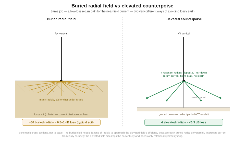
Buried radials are the right call when the vertical is ground-mounted with genuine horizontal real estate to spare, the soil is diggable (not solid rock or a paved surface), and — this is the case elevated radials cannot serve well — the installation is a multi-band trap or fan vertical. A buried field is not resonant, so it presents essentially the same low-resistance return path at 40 m, 20 m, and 10 m simultaneously; an elevated field, being a tuned quarter-wave structure, is inherently single-band unless the builder deploys a separate resonant radial set (or a switched/relay-selected set) per band, which multiplies the mechanical complexity fast. For a Hustler-style trap vertical or a GAP-style parallel-resonator vertical (both covered in the volume ahead), a buried field sized per §6 is the conventional and correct choice.
Elevated radials are the right call when the site cannot support a buried field at all — a roof mount, a mast above a paved or rocky surface, a tower-base installation with no clear ground around it — or when the operator is running a genuinely single-band (or single-band-at-a-time, manually re-cut) vertical and wants the best efficiency the least amount of wire can buy. The height requirement is real: the radials need enough clearance above the actual earth (typically a meaningful fraction of a wavelength) that their own near-field does not couple back down into the lossy ground beneath them and reintroduce the very loss mechanism they exist to avoid — an elevated radial slung a few centimetres above wet grass is not meaningfully “elevated” in the sense this section means. Once that clearance is met, four radials sloped downward (the slope angle simultaneously tuning the feedpoint impedance toward 50 Ω, as Vol 1 develops) is the standard, well-proven configuration, and it is the one the DIY build later in this dive walks through step by step.
The table below collects the deciding constraints in one place:
Table 2 — The table below collects the deciding constraints in one place
| Favors buried radials | Favors elevated radials |
|---|---|
| Ground-mounted vertical, space to spare | Roof, tower, or mast mount above obstructions |
| Diggable soil | Rocky, paved, or otherwise inaccessible ground |
| Multi-band trap or fan vertical | Single-band (or one-band-at-a-time) operation |
| Willing to invest labor for the last half-dB | Wants the best efficiency-per-radial, minimal wire |
| Soil is only average-to-good (elevated can’t fix bad far-field ground, §3) | — |
That last row is worth flagging explicitly because it is the mistake the choice most often produces: neither a buried nor an elevated radial system touches the §3 pseudo-Brewster degradation at all. Both systems solve the near-field return-current problem this section has been quantifying; neither can buy back gain lost to poor far-field ground quality, because that loss happens in the reflection the radiated wave itself makes off the earth well beyond the radial field’s own footprint. A perfect elevated radial system on genuinely poor (dry, sandy, or rocky) soil is still subject to the reduced peak gain and lifted takeoff angle §3’s table quotes for that soil class — it will be an efficient antenna radiating into a degraded pattern, which is a real improvement over an inefficient antenna radiating into the same degraded pattern, but it is not a cure for the site’s underlying ground quality. The two problems are genuinely independent, and treating a radial upgrade as a fix for a poor-soil pattern problem is a category error worth avoiding.
2.9 SWR, bandwidth, and the low-SWR trap
Vol 1’s feedpoint discussion already flagged the single-frequency version of a counterintuitive trap: a vertical with a mediocre or absent radial field can show a better SWR at resonance than a well-grounded one, because ground loss adds a resistive component that lifts the feedpoint toward 50 Ω from below. This section develops the same trap across frequency, and the mechanism is sharper — and more diagnostic — than the single-frequency version, because it explains an entire SWR curve rather than just its minimum value.
The governing relationship is the same one that sets any resonant antenna’s 2:1-SWR bandwidth: on a line matched to the antenna’s resonant resistance R, the SWR reaches 2:1 when the feedpoint reactance magnitude reaches |X| = 0.707·R (the algebra: SWR 2 corresponds to a reflection-coefficient magnitude |Γ| = 1/3, and |Γ|² = X²/(4R² + X²) = 1/9 solves to |X| = R/√2). Moving off resonance, the reactance grows at a rate — dX/df — set by the antenna’s physical geometry (the element’s length-to-diameter ratio, exactly as it is for a dipole) and essentially unaffected by how much series loss resistance sits in the circuit, because R_loss is a real, non-reactive term that does not change how fast the element’s own stored reactive energy swings with frequency. The 2:1-SWR bandwidth is the frequency span over which the rising reactance crosses ±0.707·R, and since R = R_rad + R_loss while dX/df stays essentially fixed, the 2:1 bandwidth scales up directly with the total resistance at the feedpoint — which means it scales up directly with ground loss.
Running a concrete comparison makes the size of the effect obvious. Take a 20 m quarter-wave vertical built from ½″ tubing, whose 2:1-SWR bandwidth over a well-grounded feedpoint (R ≈ 36–45 Ω, per Vol 1’s good-radial-system figures) runs in the 6–8% range quoted for that construction elsewhere in this dive. Move the same physical antenna to poor soil with a token radial field, where §5’s numbers put R_loss at a hundred-plus ohms and the total feedpoint resistance near 140–180 Ω — roughly triple to quadruple the well-grounded case — and the 0.707·R threshold triples or quadruples right along with it. Since dX/df has not changed (it is the same physical tubing element), the frequency span needed to reach that threshold widens by roughly the same factor: a 6–8% bandwidth antenna reads as 18–30%+ on the sweep, an SWR curve so broad and flat it looks, to anyone reading only the meter, like an exceptionally well-engineered wideband design. It is nothing of the kind. The width is bought entirely with radiated power converted to soil heat, and the honest 36–45 Ω feedpoint of a properly grounded installation, sitting closer to the coax’s native impedance, both looks narrower on the sweep and radiates far more of what you send it.
The diagnostic upshot deserves to be stated as plainly as Vol 1 stated the single-frequency version: a suspiciously broad, flat, forgiving SWR curve on a ground-mounted vertical is not evidence of a good match — it is one of the clearest available symptoms of a bad ground system. A properly built quarter-wave vertical over a competent radial field has a genuinely narrow-ish 2:1 window, the same order as any other resonant HF element of similar length-to-diameter ratio, and that narrowness — not the broad, undemanding sweep of a lossy installation — is what a builder should expect and want to see. Where the two SWR curves genuinely cannot be told apart is at the single frequency of best match; it is the width of the curve, not its minimum value, that carries the efficiency information, which is exactly why this section exists as the frequency-domain companion to Vol 1’s single-frequency version of the same trap.
2.10 Where this volume hands off
This volume took the feedpoint Vol 1 established and worked out where the power actually goes and how much of it survives the trip. On the pattern side: the perfect-ground elevation lobe peaking at a genuine 0° elevation and 5.15 dBi (§2), the physical reason real, lossy ground cannot sustain that peak — the pseudo-Brewster degradation of the vertically-polarized Fresnel reflection coefficient — quantified from salt water’s near-ideal behaviour down through typical and poor soil’s several-dB, several-tens-of-degrees penalty (§3), and the omnidirectional azimuth circle with its real-world 2–5 dB distortion from asymmetric radial layout or nearby conductive structures (§4). On the radial-field efficiency side — the section this dive is built around — the η = R_rad/(R_rad + R_loss) formalism (§5), the diminishing-returns curve that makes 60 buried radials the practical amateur ceiling and explains why in parallel-resistance terms (§6), the elevated-radial result that four resonant counterpoise wires beat that buried field by sidestepping lossy earth entirely rather than merely intercepting current from it (§7), and the site-driven decision between the two (§8). On the frequency side: the mechanism by which ground loss inflates the 2:1-SWR bandwidth, and the trap it sets for anyone who reads a broad, flat SWR sweep as a sign of quality rather than a sign of loss (§9).
The fixed-vertical story continues from here into the hardware that puts these numbers to work. The full-size multi-band trap verticals and the half-square gain booster — where the buried-radial requirement of §6 and §8 is the conventional choice precisely because those designs are multi-band — are next in this dive. The shortened and loaded verticals that follow them pay a second, independent efficiency tax on top of everything this volume covers — the Chu-Harrington-bounded loading-coil loss of an electrically short element — and the best-case and worst-case siting guidance and power-handling limits round out the theory side of the dive. The hands-on build volume takes the elevated-ground-plane configuration this volume developed the physics for and turns it into a step-by-step construction with a NanoVNA sweep that reads exactly the widened-or-narrow SWR curve §9 predicts, plus the commercial-buy survey and the practical radial-installation procedure — wire gauge, bonding hardware, burial depth — that this volume deliberately left to the builder’s volume rather than duplicating here.
2.11 Resources
- ARRL Antenna Book (25th+ ed.), the verticals and grounding chapters — the canonical amateur reference for the ground-quality-versus-gain tables, the buried-radial diminishing-returns data, and the elevated-radial matching guidance used throughout this volume.
- Brown, G. H., Lewis, R. F., and Epstein, J., “Ground Systems as a Factor in Antenna Efficiency,” Proceedings of the IRE, 1937 — the original experimental broadcast-ground-system study behind the buried-radial diminishing-returns curve and the historical “120 radials” broadcast standard.
- Severns, Rudy (N6LF), “Experimental Determination of Ground System Performance for HF Verticals” and the related elevated-vs-buried-radial NEC modeling series (QST / antennasbyn6lf.com) — the modern confirmation and refinement of the Brown-Lewis-Epstein result, and the primary modern source for the elevated-radial efficiency figures used here.
- Balanis, Antenna Theory: Analysis and Design (4th ed.) — the Fresnel reflection-coefficient derivation for a lossy dielectric half-space, the pseudo-Brewster-angle behaviour for parallel (vertical) polarization, and the image-theory treatment of a monopole over a finite-conductivity ground.
- ON4UN, Low-Band DXing (5th ed.) — the standard low-band operator’s reference for ground-quality effects on vertical antenna performance and radial-system design tradeoffs at 80/160 m.
- L. B. Cebik (W4RNL) antenna-modeling papers — extensive NEC-modeled treatment of vertical antennas over real ground, ground-quality-versus-takeoff-angle curves, and the buried-versus-elevated radial comparison, archived across the antenna-modeling community.
- Maxwell, Walter (W2DU), Reflections III — the standard clarification of the SWR/efficiency relationship this volume’s §9 depends on; the same “SWR does not measure efficiency” argument Vol 1 makes at a single frequency, developed here across the full sweep.
Comments (0)