The Quarter-Wave Monopole — Image-Plane Theory & Feedpoint

---

1.1 About this volume

Of all the antennas in this hub, the quarter-wave monopole is the one whose theory hides the most inside the one piece of hardware you cannot see. The visible antenna is a single conductor, a quarter-wavelength tall, fed at its base — simpler geometry than a dipole, which needs two symmetric arms and a center feed. But that apparent simplicity is a trick of visibility. The monopole only behaves like a resonant radiator because the ground beneath it is doing exactly half the antenna’s job, supplying — electromagnetically, not physically — the other quarter-wavelength that would otherwise have to be there. Understand that missing half correctly and every number this family of antennas produces (the 36 Ω feedpoint, the 5.15 dBi gain figure that gets misquoted constantly, the low-angle pattern that is the vertical’s entire reason for existing) falls out of one clean derivation. Get it wrong — treat the ground as scenery rather than as half the antenna — and you will spend a career being surprised by verticals that “should” work and don’t.

This volume owns the foundational physics: the method-of-images derivation that makes a monopole-over-ground equivalent to a free half-wave dipole, the 234/f_MHz length rule that derivation implies, the standing-wave current and voltage distribution on the element, the 36 Ω radiation resistance and the 5.15 dBi directivity-over-perfect-ground that both fall out of the same halving argument, and the feedpoint matching question — what the 36 Ω/50 Ω mismatch costs you (essentially nothing) and what the real matching options are when it costs you more than that. What this volume deliberately does not do is treat the ground as a perfect conductor and stop there. Section 6 breaks that idealization open just far enough to introduce ground-loss resistance and the efficiency relation η = R_rad/(R_rad + R_loss) — the single equation that governs whether a given vertical installation is a DX performer or a very well-engineered space heater — and then hands the full radial-system treatment, together with the radiation pattern this same geometry produces (the low-angle advantage, the elevation-versus-soil-quality table, the azimuth behavior near real obstacles), to Vol 2, where both belong. The full-size multi-band HF trap verticals that dominate the commercial market, and the half-square, are Vol 3’s subject. Shortened and loaded verticals, the efficiency penalty loading imposes, and a decision guide across the whole vertical family are Vol 4. The DIY build and the commercial-buy survey are Vol 5. Everything downstream leans on the image-plane derivation this volume establishes first.

The reader is assumed to already own the single-band dipole reference dive’s vocabulary — the standing-wave picture, the trim factor, the 73 + j42.5 Ω free-space feedpoint, the 2.15 dBi/0 dBd directivity reference. That dive is the closest sibling this one has, and the derivation here is, quite literally, half of that one.

1.2 The image-plane derivation — a monopole is half a dipole

Start from the electromagnetic boundary condition that makes a ground plane useful in the first place: a perfect electric conductor (PEC) requires the tangential electric field at its surface to be zero. The method of images is the standard trick for satisfying that condition without solving the boundary-value problem directly — you remove the conductor, and replace it with a fictitious “image” source, positioned as the mirror reflection of the real source, whose field exactly cancels the real source’s tangential field at the plane where the conductor used to be. Get the image’s position, magnitude, and phase right, and the combined field of [real source + image] automatically satisfies the boundary condition everywhere on the plane — which means it is the solution above the plane, by uniqueness.

The phase of the image current is the detail that separates two cases that are easy to confuse, and it is worth being precise about it because the wrong intuition is common. For a current element oriented parallel to the ground plane (a horizontal wire above earth — the situation the single-band dipole dive treats when it discusses height-dependent feedpoint impedance), the image current runs in the opposite direction to the real current. For a current element oriented perpendicular to the ground plane — exactly the monopole’s geometry, current flowing straight up the mast — the image current runs in the same direction as the real current. Both rules exist to force the same boundary condition (zero tangential E at the surface); they come out with opposite signs because the geometry relating “tangential” to “vertical” flips between the two orientations. The practical consequence for a vertical is immediate and favorable: the image reinforces rather than cancels.

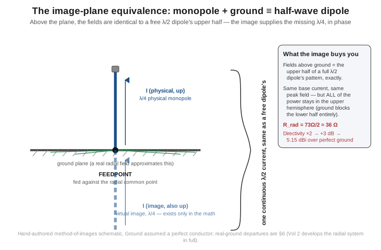
Apply this to a quarter-wave monopole standing on a ground plane, fed at its base. Set up coordinates with the ground at z = 0 and the monopole running from z = 0 to z = λ/4. Its image is a virtual quarter-wave element running from z = 0 down to z = −λ/4, carrying current in the same direction (both “outward,” away from the feedpoint, in the sense that matters for the boundary condition). Physical element plus image together form a single continuous conductor from −λ/4 to +λ/4 — exactly λ/2 long, fed at its center (z = 0) — which is precisely the geometry of the canonical half-wave dipole. Because image theory guarantees the combined field satisfies the ground’s boundary condition and matches the free-space field of that equivalent dipole above the plane, the field the monopole-over-ground produces for z > 0 is identical, point for point, to the field a full half-wave dipole would produce in its own upper half-space, driven by the same base current.

That last clause is the whole derivation, and it is worth sitting with the two things it says. First, the field strength is unchanged — the monopole radiates exactly as strongly, in every upper-hemisphere direction, as the equivalent dipole would. Second, and this is the part that produces the interesting numbers, the ground has physically deleted the lower hemisphere. A free dipole radiates its power into a full sphere, split symmetrically between the hemisphere above its equatorial plane and the hemisphere below — the dipole’s far-field pattern factor, E_θ ∝ cos((π/2)cos θ)/sin θ measured from the wire axis, is an even function of cos θ and therefore radiates exactly half its total power into each hemisphere. A monopole over a perfect ground plane produces the identical upper-hemisphere field, but there is no lower hemisphere left to carry the other half of the power away — the PEC ground reflects everything that would have gone down, and by the uniqueness of the field solution above the plane, that reflected contribution is already accounted for inside the upper-hemisphere field you just computed. Nothing new is radiated downward and nothing is radiated at all below the plane. All of what would have been the dipole’s total radiated power is concentrated into the same half-space that used to carry only half of it, at the same field strength. This is the source of both headline numbers in this volume, and the next two sections extract them cleanly.

1.3 Deriving the 234/f quarter-wave length

Before turning to impedance and gain, it is worth nailing down the physical length, because the derivation is inherited wholesale from the dipole and the reader should see why. A monopole conductor plus its image forms exactly the same λ/2 structure the single-band dipole dive analyzed, cut short of a full free-space half-wavelength by the same end-effect — the shunt capacitance at the open, high-voltage tip that makes the physical conductor electrically longer than its bare length, so it must be trimmed shorter to land on resonance. The physical monopole is one leg of that dipole, and one leg’s trim factor is the same trim factor, because the physics producing it (tip capacitance, finite conductor diameter, reduced propagation velocity along the wire) does not care whether the other leg is a real conductor above ground or a virtual image below it.

Starting exactly as the dipole derivation does: the free-space wavelength in feet is λ_feet ≈ 984/f_MHz (from c ≈ 9.836 × 10⁸ ft/s), so a free-space quarter-wavelength is

(λ/4)_feet = 246/f_MHz.

Apply the same thin-wire trim factor, k ≈ 0.95, that a #14-class HF element uses:

L_feet = 0.95 × 246/f_MHz = 233.7/f_MHz ≈ 234/f_MHz.

This is exactly the per-leg constant the dipole’s 468/f_MHz total-length formula already contains — 468/2 = 234 — which is not a coincidence but a restatement of the fact that a monopole is one leg of the equivalent dipole, cut by the same rule. The metric form follows the same way: λ_m = 300/f_MHz, the free-space quarter-wave is 75/f_MHz, and at k ≈ 0.95 the physical length is ≈ 71.3/f_MHz meters — the same constant the dipole’s per-leg metric figure produces.

The trim factor is not a universal constant; it depends on the conductor’s length-to-diameter ratio exactly as it does for a dipole leg, and a fatter monopole element (aluminum tubing rather than wire) needs a smaller k because its greater diameter concentrates more shunt capacitance at the tip relative to its length. The table below applies k = 0.95 (thin #10-class wire) and k = 0.93 (1/2″-class tubing, the standard amateur ground-plane build) across the HF bands, using the design frequencies that also anchor this hub’s other volume-length tables:

Table 1 — The trim factor is not a universal constant; it depends on the conductor's length-to-diameter ratio exactly as it does for a dipole leg, and a fatter monopole element (aluminum tubing rather than wire) needs a smaller k because its greater diameter concentrates more shunt capacitance at the tip relative to its length. The table below applies k = 0.95 (thin #10-class wire) and k = 0.93 (1/2″-class tubing, the standard amateur ground-plane build) across the HF bands, using the design frequencies that also anchor this hub's other volume-length tables

Band	Design freq	λ/4 free-space	Cut at k = 0.95 (#10 wire)	Cut at k = 0.93 (1/2″ tubing)
160 m	1.900 MHz	39.47 m (129.5 ft)	37.50 m (123.1 ft)	36.71 m (120.5 ft)
80 m	3.650 MHz	20.55 m (67.4 ft)	19.52 m (64.0 ft)	19.11 m (62.7 ft)
60 m	5.358 MHz	13.99 m (45.9 ft)	13.29 m (43.6 ft)	13.01 m (42.7 ft)
40 m	7.150 MHz	10.48 m (34.4 ft)	9.96 m (32.7 ft)	9.75 m (32.0 ft)
30 m	10.125 MHz	7.40 m (24.3 ft)	7.03 m (23.1 ft)	6.88 m (22.6 ft)
20 m	14.175 MHz	5.29 m (17.4 ft)	5.03 m (16.5 ft)	4.92 m (16.1 ft)
17 m	18.118 MHz	4.14 m (13.6 ft)	3.93 m (12.9 ft)	3.85 m (12.6 ft)
15 m	21.225 MHz	3.53 m (11.6 ft)	3.36 m (11.0 ft)	3.28 m (10.8 ft)
12 m	24.940 MHz	3.01 m (9.86 ft)	2.86 m (9.37 ft)	2.80 m (9.18 ft)
10 m	28.500 MHz	2.63 m (8.63 ft)	2.50 m (8.20 ft)	2.45 m (8.04 ft)
6 m	50.250 MHz	1.49 m (4.89 ft)	1.42 m (4.65 ft)	1.39 m (4.55 ft)

Read the same caution the dipole dive gave the analogous table: 234/f (or its k-adjusted variants here) is a starting cut, not a final dimension. The formula assumes an idealized thin-wire or moderate-tubing element in isolation; a real installation’s exact resonant length depends on the base hardware’s capacitance to the radial system, nearby metal, and the conductor’s actual diameter profile if it tapers or telescopes. The correct procedure — identical to the dipole’s — is cut long, hoist, sweep with an analyzer, and trim; that workflow is developed hands-on in Vol 5.

1.4 The standing-wave picture — current at the base, voltage at the tip

The current and voltage distributions on the monopole are not new physics; they are exactly one quarter of the dipole’s cosine/sine standing wave, because the monopole is exactly one quarter of that structure (the other quarter being the image, which does not carry a physical current you could touch but which the math treats identically). Using the same z-along-the-element convention as §2, with z = 0 at the base (feed) and z = λ/4 at the tip, and β = 2π/λ:

I(z) ≈ I₀ · cos(βz) and V(z) ≈ V₀ · sin(βz),

valid for 0 ≤ z ≤ λ/4. At the base, cos(0) = 1: the current is at its maximum, exactly the value the equivalent dipole would show at its center feedpoint. At the tip, cos(π/2) = 0: the current falls to zero, because the tip is an open circuit and no current can flow off the end of a wire into free space. The voltage runs the complementary path — sin(0) = 0 at the base, rising to sin(π/2) = 1, its maximum, at the tip.

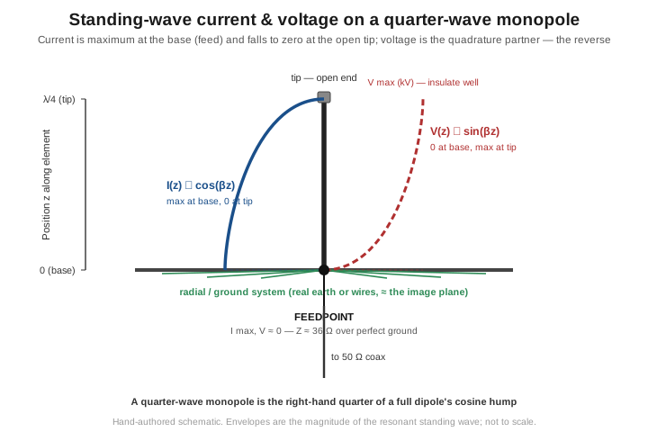
Two practical consequences fall directly out of this picture, and they are the mechanical mirror of the dipole’s feedpoint-versus-ends distinction, just relocated. The base is where the current lives, and it wants conductivity. This is where the feed happens (naturally — you feed a resonant structure at its current maximum for the same reason a dipole is fed at center), and it is also where the radial or ground system attaches. Any resistance in that connection — a corroded radial-to-mast bond, an undersized common-point bus, a poorly-terminated coax shield — dissipates real I²R power exactly where the current is largest, which is precisely why §6 treats the base connection as load-bearing rather than incidental. The tip is where the voltage lives, and it wants dielectric strength. At legal amateur power the tip of a quarter-wave vertical carries a standing-wave voltage in the low kilovolts, exactly as the ends of a dipole do — which is why the top of a vertical, whether it terminates in bare wire, a capacitive top-hat (a deliberate exploitation of this high-voltage point, covered in Vol 4), or simply thin air, needs to be kept clear of nearby grounded metal and foliage that could arc or detune it.

The base-feed geometry also explains, without any further derivation, why a monopole is naturally a low-impedance, high-current feed in a way a center-fed dipole is not quite the same: the monopole’s entire feed happens at the single point where the standing wave is at its current antinode, whereas a dipole splits that same current antinode across two symmetric arms meeting at a shared center. The monopole’s feedpoint impedance is therefore referenced to the same current-maximum convention the dipole dive used, and the next section shows exactly what that impedance is and why.

1.5 Radiation resistance and gain — why 36 Ω buys you 5.15 dBi

§2 established the physical picture; this section turns it into the two numbers every quarter-wave vertical is built around. Both fall out of the same fact — same field strength, half the radiated power — applied to two different definitions.

Radiation resistance is defined, as in the dipole dive, by R_r = P_rad/|I|² referenced to the feedpoint current. A free half-wave dipole, fed with current I₀ at its center, radiates a total power P_dipole = |I₀|² · 73 Ω (the canonical thin-dipole figure). Because that power splits evenly between the dipole’s two hemispheres, the power it puts into its upper half-space alone is P_dipole/2 = |I₀|² · 36.5 Ω. The monopole-over-ground, fed with the same base current I₀, produces that identical upper-hemisphere field — and because the ground has deleted the lower hemisphere entirely, all of the monopole’s radiated power is that upper-hemisphere contribution:

P_monopole = |I₀|² · 36.5 Ω, so R_r(monopole) = P_monopole/|I₀|² = 73/2 ≈ 36 Ω.

This is the canonical figure this hub’s earlier flat treatment quoted, and it is the correct, derivable number for a quarter-wave element over an idealized perfect ground: ≈ 36 Ω of radiation resistance, referenced to the base current, half the dipole’s 73 Ω because the monopole only ever had to build up the current distribution across half the conductor length the dipole uses, for a given radiated field.

Gain follows the same halving argument applied to directivity rather than resistance, and it is worth working through explicitly because the arithmetic is where the “5.15 dBi” figure most often gets garbled in casual explanations. Directivity is defined as D = 4π U_max / P_rad, where U_max is the peak radiation intensity (power per solid angle) in the antenna’s favored direction. For both the dipole and the monopole, that peak occurs broadside — at the horizon, θ = 90° from the wire axis — and because the monopole’s upper-hemisphere field is identical to the dipole’s, U_max is the same number in both cases. What differs is only the denominator: the dipole’s D = 1.64 (the familiar 2.15 dBi) uses the dipole’s full radiated power P_dipole, while the monopole’s directivity uses P_monopole = P_dipole/2:

D(monopole) = 4π U_max / (P_dipole/2) = 2 × [4π U_max / P_dipole] = 2 × D(dipole) = 2 × 1.64 = 3.28.

Converting to decibels, 10 · log₁₀(3.28) ≈ 5.16 dBi, universally quoted (and reproduced here) as 5.15 dBi — the canonical monopole-over-perfect-ground directivity figure appearing throughout the ARRL Antenna Book, Balanis, and Kraus. The reasoning behind the number is worth restating in one sentence because it resolves a persistent point of confusion: the monopole is not “3 dB better” because it radiates more strongly in any given direction — it radiates with the same peak field strength as the dipole — it is 3 dB better because the same peak field is now carrying twice the fraction of a (halved) total radiated power, an artifact of concentrating all of a smaller total power budget into a hemisphere that used to share it with a twin. Halving the denominator while holding the numerator fixed doubles the ratio; doubling a linear directivity ratio is +3.01 dB, hence the familiar shorthand “2.15 dBi + 3 dB = 5.15 dBi.”

Two qualifications, both flagged here and developed fully downstream, keep this honest. First, 5.15 dBi is a perfect-ground number — it assumes the idealized PEC image-plane derivation of §2 all the way through, and no real amateur installation sits over a perfect conductor. Real ground absorbs some of the near-field return current as heat and imperfectly reflects the far-field wave, both of which reduce the achievable peak gain below 5.15 dBi — often substantially, depending on soil and radial-system quality, as §6 begins to quantify and Vol 2 develops in full. The figure is real physics, not a marketing number, but it is a ceiling, reached only in the neighborhood of salt-water grounding and a properly executed radial or elevated-counterpoise system — never assume it as a default. Second, like the dipole’s 2.15 dBi, this is a directivity, and it converts to gain only to the extent the antenna is efficient; §6 is exactly where directivity and gain start to part company for a real vertical.

1.6 Real ground breaks the image — loss resistance and the efficiency it costs

Every number in §§2–5 assumed a perfect electric conductor beneath the monopole, and no such thing exists outdoors. Real soil is a lossy dielectric with finite conductivity — figures spanning roughly 10⁻⁴ S/m for very dry sand or desert soil up through 10⁻²–10⁻¹ S/m for damp farmland and approaching 5 S/m for seawater — and current that would, over a perfect image plane, flow losslessly through the “ground” instead flows through real earth and dissipates as I²R heat. This heating happens in the near-field return-current region directly beneath and around the antenna, exactly where the base-fed current of §4 has to complete its circuit back to the feedpoint. A radial system’s entire purpose is to intercept that return current before it dives into lossy soil and instead route it back through low-resistance metal — replacing the real ground, in the near field, with something closer to the ideal image-plane conductor the derivation assumed. How well a given radial field does that job is Vol 2’s whole subject; this section only needs to establish where the loss enters the circuit and what it costs.

The place it enters is exactly where you would expect from the standing-wave picture: in series with the radiation resistance, at the feedpoint. The base is the current antinode; the return current from the radial system rejoins the circuit there; and whatever resistance that return path carries — soil resistance in the near-field zone, contact resistance at radial-to-mast bonds, the resistance of the radial wire itself — appears as an honest series resistor stacked on top of the R_rad ≈ 36 Ω this volume derived. Call that series term R_loss. The feedpoint the antenna analyzer actually measures is not R_rad alone; it is

R_feed = R_rad + R_loss.

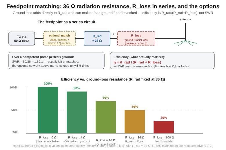
That series relationship has an immediate and important consequence for efficiency. Only R_rad represents power actually leaving the system as radiation; R_loss represents power leaving the system as heat in the ground. For the same feedpoint current, the fraction of the total input power that is radiated — the radiation efficiency — is exactly the ratio of the two resistors:

η = R_rad / (R_rad + R_loss).

This is the standard antenna-efficiency relation (Balanis and Kraus both develop it in exactly this form, for any antenna where the loss can be modeled as a series resistance at the current reference point), and for a quarter-wave vertical it is the single equation that governs whether the 5.15 dBi ceiling of §5 is anywhere close to achievable. With R_rad = 36 Ω fixed by the geometry, the efficiency curve is steep: a radial field good enough to hold R_loss down to 4 Ω (roughly the territory of 60-plus buried radials over decent soil) yields η = 36/40 = 90% — a loss of well under half a dB. A sparser field that leaves R_loss around 16 Ω costs η = 36/52 ≈ 69% — a real, audible-on-the-margin 1.6 dB. And an installation with R_loss = 36 Ω — loss resistance equal to the radiation resistance itself, not a hypothetical extreme but a realistic number for a ground-mounted vertical with only a handful of short radials over ordinary soil — is at η = 50%, meaning half of every watt the transmitter delivers to the feedpoint becomes soil heating rather than a signal on the air, a full 3 dB of gain quietly given away before the radiation-pattern physics of Vol 2 ever gets a say. Push R_loss to 100 Ω — plausible for a vertical with no radial system worth the name — and η falls to 26%, better than 5.8 dB below where the antenna’s own geometry says it should be.

The efficiency relation also explains a counterintuitive fact that every serious vertical installer eventually runs into: a mediocre radial field can produce a better-looking SWR than a good one, for exactly the wrong reason. R_loss adds directly to R_rad, lifting R_feed toward — and sometimes past — the 50 Ω a coax feedline wants to see, so a vertical with too few radials can present a flatter SWR curve than the same vertical with a properly engineered radial field, purely because the ground loss is doing the matching network’s job by burning the mismatch off as heat instead of reflecting it. SWR is a measurement of the feed system’s bookkeeping, not of how much of the input power left as radiation; it cannot distinguish “well-matched because R_rad and the line impedance are close” from “well-matched because R_loss dragged a mismatched R_rad up to meet the line.” This is precisely why Vol 2 exists as its own volume rather than a footnote here: the radial (or elevated-counterpoise) system is not incidental hardware, it is the component that sets R_loss, and R_loss is the term that decides whether this volume’s 36 Ω and 5.15 dBi are numbers you actually get to use or numbers you are heating your backyard with instead.

1.7 The 36 Ω feedpoint on 50 Ω coax

Set the ground-loss question aside for a moment and return to the idealized case — a quarter-wave monopole over a near-perfect ground (a genuinely excellent radial or elevated-counterpoise system, close enough to the image-plane assumption that R_loss is small next to R_rad) — because the pure impedance-matching arithmetic is worth doing on its own, exactly as the dipole dive did for its 73 Ω figure. At resonance (the reactance trimmed to zero by the length adjustment of §3), the feedpoint presents

Z_fp ≈ 36 + j0 Ω.

Feeding that with ordinary 50 Ω coax gives a reflection coefficient

Γ = (36 − 50)/(36 + 50) = −14/86 ≈ −0.163,

and a voltage standing-wave ratio

VSWR = (1 + |Γ|)/(1 − |Γ|) = 1.163/0.837 ≈ 1.39:1.

That figure — 1.39:1, sometimes quoted as “1.4:1” — is the entire native mismatch of a textbook quarter-wave vertical on 50 Ω coax, and it should look immediately familiar: it is the same size mismatch (|Γ| ≈ 0.16–0.19, VSWR in the 1.4–1.5:1 range) that the dipole dive found for its own 73 Ω-on-50-Ω case, because both are instances of the same generic “canonical antenna impedance a few tens of ohms off the standard coax impedance” situation, just approached from opposite directions — the dipole runs high of 50 Ω, the monopole runs low. The forward power reflected at the junction, |Γ|² ≈ 0.027, is under 3%, and the resulting mismatch loss,

ML = −10·log₁₀(1 − |Γ|²) ≈ 0.12 dB,

is, exactly as for the dipole, inaudible and operationally irrelevant. Every argument the dipole dive made about why chasing a perfect 1:1 is effort without payoff applies here without modification: a modern solid-state HF transceiver delivers full rated power into a 1.4:1 load without any protection-circuit foldback (which typically does not engage until somewhere around 2:1–3:1), the reflected energy is not simply thrown away but largely re-reflected and eventually radiated on a low-loss line, and the residual genuine dissipation under this modest a standing wave is a few hundredths of a dB at most. For a resonant quarter-wave vertical over a competent ground system feeding a modern radio through reasonably short, low-loss coax, no matching network is required at all — the single most common unforced complication in amateur vertical installations is reaching for a transformer that a 1.39:1 SWR never actually needed.

The place this arithmetic goes wrong is not the coax junction; it is upstream, at the antenna itself, when R_loss from §6 has shifted the actual feedpoint resistance away from the idealized 36 Ω this section assumed. A ground-mounted vertical over a sparse radial field genuinely presents something closer to 60–90 Ω, not because the antenna’s geometry has changed but because R_loss has been added in series — and that feedpoint, not the clean 36 Ω, is what a 50 Ω line actually sees. It bears repeating from §6: an elevated SWR reading in that situation is telling you about ground loss, not about a geometry problem that a matching network would fix, and reaching for a transformer to “clean up” that SWR without first addressing the radial system treats the symptom while leaving the actual efficiency loss — the power you are burning in the dirt — completely untouched.

1.8 Matching the feedpoint — gamma, hairpin, unun, and the quarter-wave transformer

Given §7’s conclusion that a resonant vertical over a decent ground system rarely needs matching, when does reaching for a network make sense, and what are the honest options? Three situations justify it: an installation where the feedpoint resistance really has drifted meaningfully from 36 Ω (elevated radials sloped at an angle that deliberately targets 50 Ω, discussed below, or a shortened/loaded element whose resistance behaves differently — Vol 4’s subject); a feedline long or lossy enough that the additional-loss-under-SWR term (the same effect the dipole dive quantified) is no longer negligible; or simply an operator who wants the SWR meter to read closer to 1:1 for its own sake, which is a legitimate aesthetic preference as long as it is not mistaken for an efficiency improvement. Four matching topologies cover essentially all of practical vertical-antenna work:

The shunt-feed / gamma match taps the coax’s center conductor onto the vertical element some distance up from the base rather than at the base itself, with a series capacitor tuning out the reactance the tap introduces. This is the standard solution for verticals that are not electrically isolated from a grounded structure at the base — a grounded tower used as a vertical radiator, for instance, where you cannot insert an insulated base feedpoint at all. The tap point acts as an impedance transformer: moving it higher up the element (toward the current maximum) lowers the impedance seen at the tap, and moving it lower (toward the base, where a driven monopole is already at its current maximum) raises it, so the gamma match’s tap position is chosen to land on 50 Ω resistive once the series capacitor cancels the reactance the offset feed introduces. It is a single-band, narrowband solution — exactly the tradeoff the equivalent Yagi driven-element gamma match makes — and its main appeal for verticals specifically is that it requires no insulated break at the base at all.

The hairpin / beta match is the vertical-antenna analog of the technique more commonly associated with Yagi driven elements: a shorted shunt inductor (the “hairpin,” a U-shaped piece of wire or tubing) connected across the feedpoint cancels a capacitive reactance the antenna presents when it is fed slightly short of resonance, while simultaneously stepping the resistive part up toward 50 Ω. It is most relevant for a vertical deliberately cut a little short of resonance (trading a small, easily-matched capacitive reactance for a feedpoint resistance closer to 50 Ω than the resonant 36 Ω would be) — a legitimate design choice, but one that requires understanding the resistance-versus-length relationship well enough to land the hairpin’s compensation correctly, and it is workable bench-top engineering rather than a drop-in part.

A step-up transmission-line transformer (unun) is the most drop-in of the four options for the plain case of “the feedpoint really is close to 36 Ω resistive and I want 50 Ω.” Since 50/36 ≈ 1.4, a 1.5:1 unun — a small bifilar-wound transformer on a ferrite toroid, functionally the impedance-stepping cousin of the 1:1 current baluns the dipole dive develops in detail — gets close enough in practice that the residual mismatch is smaller than the 1.39:1 this section started with, and it does so broadband, with no per-band retuning. This is the cleanest fix when the antenna’s own resistance is the thing you want to move, rather than compensating for a reactance, and it is the matching device most commercial elevated ground-plane vertical kits ship with when they ship one at all.

The quarter-wave transformer (Q-section) takes a different approach entirely: rather than a lumped or wound device at the feedpoint, insert a quarter-wavelength of transmission line whose characteristic impedance is the geometric mean of the two impedances being matched, Z_Q = √(Z_ant · Z_line). For 36 Ω to 50 Ω, Z_Q = √(36 × 50) ≈ 42 Ω — inconveniently close to standard 50 Ω or 75 Ω coax, so a genuinely custom-impedance quarter-wave section (parallel runs of standard coax, or a hand-built section of the right conductor spacing) is usually the only way to hit it exactly, which is why the Q-section sees far more use matching larger impedance transformations (a folded-element feedpoint to 50 Ω, for instance) than it does cleaning up this comparatively small 36-to-50 Ω step. It is included here for completeness and because it is the textbook-correct tool for the job; in practice, for the specific 36 Ω figure this volume derives, the 1.5:1 unun gets there with off-the-shelf parts and no custom line to fabricate.

There is a fifth option worth naming even though it is really a ground-system technique rather than a feedpoint device: sloping the radials downward from horizontal. A radial system lifted off the ground and swept downward at roughly 30–45° from horizontal — the standard elevated ground-plane configuration — shifts the feedpoint resistance upward from the horizontal-radial value (closer to 25–32 Ω) toward 50 Ω as the slope angle increases, with a 45° slope landing close to a natural 50 Ω match with no transformer at all. This is not a violation of the 36 Ω derivation in §5 — it is a small, deliberate perturbation of the ideal geometry (the radials are no longer coplanar with the “ground” in the strict image-plane sense) that happens to land the resistance somewhere more convenient, at the cost of a slightly different current distribution on the radials themselves. It is genuinely the most elegant of all five options where it applies, because it costs no hardware and no bandwidth — the full mechanics of elevated-radial geometry belong to Vol 2, but the matching consequence is worth flagging here alongside the other four.

Whichever option applies, the standard 1:1 current choke that the dipole dive insists belongs at every dipole feedpoint has a role here too, though a smaller one: a vertical’s inherently asymmetric, fed-against-ground geometry does not invite common-mode current the way a balanced dipole’s forced-symmetric feed does, but a 1:1 choke at the point the coax leaves the radial common connection is still cheap insurance against common-mode pickup on an elevated installation, where the radial counterpoise is more exposed to that coupling than a ground-mounted radial field is. That choke belongs alongside whichever of the four impedance-matching options above is in use, not instead of it — they solve different problems, exactly as the dipole dive distinguished impedance matching from balance.

1.9 Where this volume hands off

This volume derived the physics that everything else in this dive rests on. The method of images showed why a quarter-wave monopole over a ground plane is electromagnetically the same object as half of a free-standing half-wave dipole — same field strength above the plane, but all of a halved total radiated power concentrated into the hemisphere that used to share it. That single fact produced both headline numbers: 36 Ω radiation resistance (half the dipole’s 73 Ω, because the monopole builds its field with half the conductor for the same current) and 5.15 dBi directivity over a perfect ground (double the dipole’s 1.64 linear directivity, because the same peak field now represents a larger fraction of a smaller total power budget — 10·log₁₀(2) ≈ 3.01 dB on top of the dipole’s 2.15 dBi). The standing-wave current and voltage distributions turned out to be exactly one quarter of the dipole’s own cosine/sine pair, which is also where the 234/f_MHz length rule came from — the same per-leg constant the dipole’s 468/f formula already contains, trimmed by the identical end-effect factor. Breaking the perfect-ground idealization introduced loss resistance in series with the radiation resistance and the efficiency relation η = R_rad/(R_rad + R_loss) that governs how much of the 5.15 dBi ceiling a real installation actually gets to keep — and showed why a flatter SWR reading can be the symptom of a worse-performing ground system rather than evidence of a better one. Finally, the arithmetic of the 36 Ω-versus-50-Ω-coax mismatch (1.39:1, a non-issue) and the real matching toolkit (gamma, hairpin, unun, Q-section, and sloped elevated radials) rounded out what a builder actually does at the feedpoint.

The story continues from the ground up, literally. Vol 2 takes the R_loss term this volume introduced and makes it the entire subject alongside the radiation pattern this same geometry produces once a real (imperfect) ground and real installation surroundings are accounted for — the low-angle DX advantage that is the entire reason to build a vertical in the first place, the elevation-angle-versus-soil-quality relationship, the vertical’s characteristic receive-noise penalty, buried-radial-count-versus-efficiency curves, elevated-counterpoise geometry and the sloped-radial match this volume flagged in §8, and the practical decision between the two radial strategies. Vol 3 covers the full-size multi-band HF trap verticals that dominate the commercial market and the half-square, a directional cousin of the plain quarter-wave. Vol 4 covers shortened and loaded verticals, the efficiency penalty loading imposes, the power-handling realities of the loading hardware, and a decision guide across the whole vertical family. Vol 5 puts all of it into a build: a step-by-step elevated quarter-wave ground-plane construction with a real bill of materials, the trim-and-sweep tuning workflow with a NanoVNA, and the ranked commercial-buy survey.

1.10 Resources

• ARRL Antenna Book (25th+ ed.), the vertical-antenna chapter — the canonical amateur reference for the image-plane derivation, the 36 Ω and 5.15 dBi figures, and the radial-system efficiency data this volume forward-references to Vol 2.
• Balanis, Antenna Theory: Analysis and Design (4th ed.) — the academic derivation of the monopole-over-ground-plane directivity via image theory, and the general antenna-efficiency relation η = R_rad/(R_rad + R_loss).
• Kraus, Antennas — the classic treatment of image theory, the monopole’s radiation resistance and directivity relative to the dipole, and radial-system loss.
• Stutzman & Thiele, Antenna Theory and Design (3rd ed.) — complementary treatment of the ground-plane monopole and its impedance behavior.