Radiation Pattern, Ground Effect and SWR

---

3.1 About this volume

Vol 1 fixed the element’s geometry and physics — the standing-wave current and voltage distributions, the accelerating-charge radiation mechanism, the 468/f trim rule, and the 2.15 dBi free-space directivity that makes the dipole the 0 dBd reference. Vol 2 took ownership of the feedpoint — the 73 + j42.5 Ω free-space impedance and both parts of it, the way real ground at finite height makes the resistance oscillate, the harmless 50 Ω-coax mismatch, and the 1:1 current balun that belongs at every dipole feedpoint. This volume takes the energy after it leaves the feedpoint and asks two questions that decide whether the antenna actually works for you: where does the power go in angle (the radiation pattern, in free space and — far more importantly — over real ground), and how does the match hold up as you move across the band (the SWR-versus-frequency curve, the 2:1 bandwidth, and the trim sensitivity that the cut-and-tune loop has to respect).

Those two questions are the practical heart of dipole work, and they are where the textbook 2.15 dBi free-space figure stops being the number you transmit with. Vol 1 already flagged that putting a dipole over ground at a finite height rearranges the pattern into lobes and lifts the peak gain toward roughly 7.8 dBi near a half-wavelength up; Vol 2 met the impedance shadow of that same height effect. Here the height story is told in full on the pattern side — the elevation lobing, the takeoff angle that falls as the antenna rises, the single high-angle lobe of a low dipole that NVIS exploits deliberately, and the gain-versus-height trade that answers “how high should I hang it” band by band. The free-space pattern is where we start, because it is the building block ground reflection acts on, but the over-ground pattern is the deliverable.

Stay aware of the lane. This volume owns the radiation pattern (free space and over ground), the gain-versus-height development, takeoff angle, the NVIS-versus-DX trade, polarization, and the SWR-versus-frequency / bandwidth behaviour. It does not re-derive the standing-wave or length math — that is Vol 1 — nor the static feedpoint-impedance and balun material — that is Vol 2 — and both are cited rather than repeated. The patterns of the mechanical and topological variants (folded, inverted-V, sloper, vertical dipole) belong to Vol 4, and the hands-on cut-long-and-trim procedure with a NanoVNA belongs to Vol 5; both are forward-referenced where they connect. Every pattern and gain figure here is a model-derived canonical shape — the NEC/ARRL-standard result for the ideal geometry — and the figures say so; real installations deviate through ground quality, surrounding objects, and feedline radiation, and the prose calls those deltas out where they matter.

3.2 The free-space pattern — donut, figure-8, and the pattern factor

In free space — no ground, no nearby conductors — a half-wave dipole radiates the pattern that falls directly out of integrating its cos(βz) current distribution against the geometric phase delay across the element, which Vol 1 carried through to the closed-form far-field pattern factor

E_θ ∝ cos((π/2)·cos θ) / sin θ,

where θ is the angle measured from the wire axis. This volume owns the development of that factor into the full three-dimensional pattern; the derivation itself stays in Vol 1. Read the factor at its limits and the whole shape appears. At θ = 90° — broadside, perpendicular to the wire — the numerator is cos(0) = 1 and the denominator is sin 90° = 1, so the field is maximum. As θ → 0° or θ → 180° — straight off either end of the wire — the numerator goes to cos(±90°) = 0 while the denominator also vanishes, and the ratio collapses to zero: a deep null directly off each end. Between those extremes the factor falls off smoothly and symmetrically about broadside.

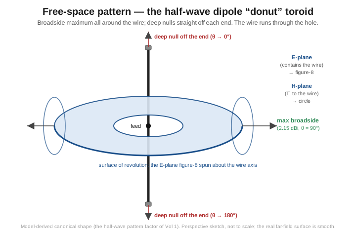
Because the factor depends only on θ (the angle from the wire) and not on the azimuthal angle around the wire, the three-dimensional pattern is a surface of revolution about the wire axis — the familiar toroid, or “donut,” with the wire threaded through the hole drawn at the head of this volume. Two orthogonal cuts through that donut are the two patterns every antenna discussion quotes, and getting their names right saves a great deal of confusion. The cut taken in any plane that contains the wire is the E-plane pattern (the plane of the electric field, which lies along the wire) — and that cut is the figure-8: two broadside lobes with the deep nulls off the ends. The cut taken in the plane perpendicular to the wire, through the feedpoint, is the H-plane pattern, and there the factor is constant — every direction in that plane is broadside (θ = 90°) — so the H-plane pattern is a circle: omnidirectional around the wire. The donut is just the figure-8 spun about the wire to sweep out the circle.

The orientation in which you hang the dipole maps these two cuts onto the directions you care about. For a horizontal dipole — the usual HF case — the plane containing the wire is the horizontal plane, so the azimuth pattern is the figure-8 (broadside maxima, end nulls), and the plane perpendicular to the wire is vertical, so the elevation pattern would be the circle were the antenna in free space. It is not in free space, and Section 5 shows how ground reflection turns that free-space elevation circle into the lobed structure that dominates a real horizontal dipole’s behaviour. For a vertical dipole the assignment swaps — the azimuth pattern becomes the omnidirectional circle and the figure-8 lies in the vertical plane — which is the geometric root of the vertical dipole’s all-around azimuth coverage taken up in Vol 4. The free-space peak directivity of all of this is the 2.15 dBi of Vol 1; the pattern simply says where that 2.15 dBi points (broadside, all around the wire) and where it does not (off the ends).

3.3 Beamwidth and the azimuth nulls

The figure-8 is a broad pattern, not a sharp beam, and quantifying “broad” is the job of the half-power beamwidth (HPBW) — the angular width of a lobe between the two directions where the radiated power has fallen to half its peak, i.e. −3 dB (a field ratio of 1/√2 ≈ 0.707). Setting the pattern factor equal to 0.707 and solving,

cos((π/2)·cos θ) / sin θ = 0.707,

gives half-power points at θ ≈ 51° and θ ≈ 129°, symmetric about the θ = 90° broadside maximum. The half-power beamwidth of the dipole’s E-plane (figure-8) lobe is therefore

HPBW ≈ 129° − 51° = 78°.

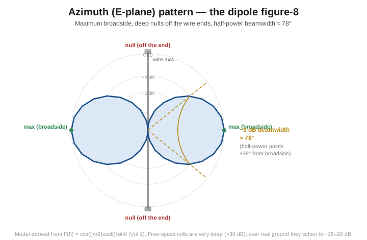
That 78° is worth carrying as a number, because it sets the practical expectation for a dipole’s directivity. A dipole is gently directional: it favours the two broadside directions by a modest margin and is down only 3 dB across a generous ±39° window, so pointing is forgiving — a dipole strung roughly broadside to your target band is within a dB or so of optimum across most of a continent’s worth of azimuth. The flip side is that the gain advantage of that broadside favouring is small (the whole free-space directivity is 2.15 dBi), so the figure-8 is a weak beam, not a substitute for a Yagi.

The nulls off the ends are the sharper and more useful feature. In free space they are very deep — well over 30 dB down, effectively a blind spot directly off each wire tip — which has two practical consequences. First, the nulls can be steered for rejection: rotating a dipole so a strong local interferer or an unwanted station falls into the end null can buy 20+ dB of suppression of that signal, and this is the basis of using a rotatable dipole as a crude direction-finding antenna (the signal disappears when the wire points at it). Second, and more often a trap, careless orientation can drop a wanted path into the null — a north-south wire has its nulls due north and south, so a station due north of you sits in the worst possible direction. The fix is to orient the wire broadside to the paths you care about most. The important real-world caveat is that the textbook >30 dB null depth is a free-space figure: over real ground the ground-reflected ray fills the nulls, and a horizontal dipole’s azimuth nulls soften to roughly 15–20 dB, deeper over highly conductive ground (salt water) and shallower over poor, dry, rocky soil. Useful for rejection, but do not expect the textbook blind spot from a wire hung over an ordinary backyard.

3.4 Polarization — linear along the wire

A dipole is a linearly polarized antenna, and the polarization is set by the simplest possible rule: the E-field is aligned with the wire. A horizontal dipole radiates horizontally polarized waves; a vertical dipole radiates vertically polarized waves; a wire strung at 45° radiates slant polarization. There is no circular or elliptical component from a straight dipole — that requires crossed elements or a helix, which live elsewhere in the hub.

The reason polarization gets attention is the cross-polarization mismatch: a receiving antenna responds to the component of the incoming field aligned with its elements, so a horizontally polarized signal arriving at a vertically polarized antenna (or vice versa) is attenuated. For ideal antennas the theoretical cross-pol rejection is infinite (the alignment is exactly zero), and in practice on a line-of-sight path — VHF/UHF, where the wave arrives with its launch polarization essentially intact — the mismatch is a real and substantial penalty, conventionally taken as on the order of 20 dB. This is why polarization discipline matters on the bands where it is preserved: VHF/UHF FM repeater and handheld work is universally vertical, and using a horizontal antenna against that infrastructure throws away most of the link; VHF/UHF weak-signal work (SSB, CW, EME, the 6 m and 2 m Yagi community) is universally horizontal, and mixing the two costs you the contact. On those line-of-sight bands, match the polarization of the station you are working, full stop.

On HF skywave, the calculus changes completely, and this is the regime where dipole users most often over-worry. A signal that has refracted through the ionosphere — passing through the birefringent, magnetized plasma and undergoing Faraday rotation, plus multipath from multiple hops and ground reflections — arrives with its polarization scrambled, the launch polarization largely randomized into a slowly rotating, effectively mixed state by the time it reaches the far end. The consequence is that the clean 20 dB cross-pol penalty of a line-of-sight path does not apply to HF skywave: a horizontally polarized transmitter and a vertically polarized receiver, both working the ionosphere, suffer only a few dB of average mismatch that fades and shifts with the path, not a fixed 20 dB. This is why an HF dipole (horizontal) and an HF vertical (vertical) work each other on skywave routinely and why the endless “horizontal versus vertical for DX” debate is really a debate about takeoff angle and ground losses (Sections 5–6), not about polarization. The honest summary is the two-regime one: on line-of-sight paths polarization matters a lot and you must match it; on HF skywave the ionosphere scrambles it and it matters far less than the takeoff-angle question that actually decides the contact.

3.5 Over real ground — the mirror and the lobes

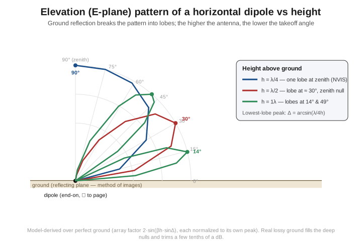
Every real horizontal dipole hangs at a finite height above real ground, and ground reflection is the dominant effect on its radiation pattern — far more consequential than the free-space figure-8, because it is what determines the elevation angles at which the antenna actually launches and receives. The cleanest model is the same method of images that Vol 2 used for the feedpoint impedance: a conducting ground plane is electrically equivalent to a mirror-image dipole an equal distance below the surface. The field at any elevation angle in the far field is then the coherent sum of two rays — the direct ray from the antenna and the ground-reflected ray, which is equivalent to the direct ray from the image. Those two rays travel slightly different path lengths to a distant observer, so they arrive with a relative phase that depends on the elevation angle and on the height, and they interfere — adding where they arrive in phase, cancelling where they arrive out of phase. The result is that the smooth free-space elevation circle breaks into a set of lobes and nulls.

For a horizontal dipole the reflected ray suffers a 180° phase reversal at the ground (the boundary condition for the horizontal E-field), and working the path-length geometry through, the elevation pattern over perfect ground is the free-space pattern multiplied by an array factor 2·|sin(βh·sin Δ)|, where Δ is the elevation angle measured up from the horizon and h is the height. That single factor explains the entire height story:

• At the horizon (Δ → 0) the factor is always zero: a horizontal dipole over ground has a null on the horizon, because the direct and ground-reflected rays cancel exactly at grazing incidence. No horizontal antenna radiates at zero elevation.
• The lowest lobe peaks where βh·sin Δ = π/2, i.e. where sin Δ = λ/(4h) — the relationship Section 6 develops as the takeoff-angle curve. The higher the antenna, the smaller that angle, so the main lobe leans progressively toward the horizon as h grows.
• At low heights — h below roughly λ/4 — the argument never reaches π/2, so there is no low lobe at all: the pattern is a single broad lobe with its maximum at or near the zenith (straight up). This is the NVIS regime of Section 7.
• As the antenna rises past about λ/2, the factor reaches π/2 at one angle and then comes back down and reaches 3π/2 at a higher angle, so additional, higher-angle lobes appear, separated by nulls (the first null lands at the zenith for h = λ/2, and at Δ = 30° for h = 1λ). The number of elevation lobes is roughly 2h/λ.

The gain bump is the second half of the ground story and the source of the numbers Vol 1 promised. At the peak of a lobe the direct and reflected rays add in phase, doubling the field; doubling the field is four times the power, which is +6 dB. Over perfect ground, then, the lobe-peak gain of a horizontal dipole is its free-space 2.15 dBi plus 6 dB, or about 8.15 dBi in the favoured direction (with the energy that would have gone into the ground and the nulls redistributed into the lobes). Real ground is not a perfect mirror — it has finite conductivity and dissipates some of the reflected energy, and the reflection coefficient is below unity — so the bump is a few tenths of a dB short of the perfect-ground ideal, which is why the canonical figure quoted for a horizontal dipole near h = λ/2 over good ground is roughly 7.8 dBi rather than the perfect-ground 8.15. That is the same ~7.8 dBi at h = λ/2 Vol 1 cited; here it is developed: it is the free-space directivity, lifted ~6 dB by coherent ground reflection at the lobe peak, discounted a few tenths by real-ground loss. The corollary that surprises newcomers is that this peak gain is fairly insensitive to height over a wide range — a horizontal dipole sits within a few tenths of a dB of ~7–8 dBi at the lobe peak from about 0.2λ to well over a wavelength — so raising the antenna does not buy you much peak gain. What it buys you is a lower takeoff angle, which is the thing that actually matters for working distance, and that is Section 6.

3.6 Takeoff angle versus height

The single practical question a dipole builder asks about height is “how high should I hang it,” and the answer is governed almost entirely by the takeoff angle — the elevation angle of the main (lowest) lobe — because that angle has to match the elevation angles at which the propagation you want actually arrives. Long-haul HF skywave (DX) arrives and leaves at low angles, typically under ~15°; regional and short-skip work uses medium-to-high angles; NVIS uses near-vertical angles. Setting the lobe-peak condition sin Δ = λ/(4h) from Section 5 gives the takeoff angle directly as a function of height in wavelengths:

Δ_peak = arcsin( λ / 4h ) for h ≥ λ/4,

with the single lobe pinned at the zenith (Δ = 90°) for any height below λ/4.

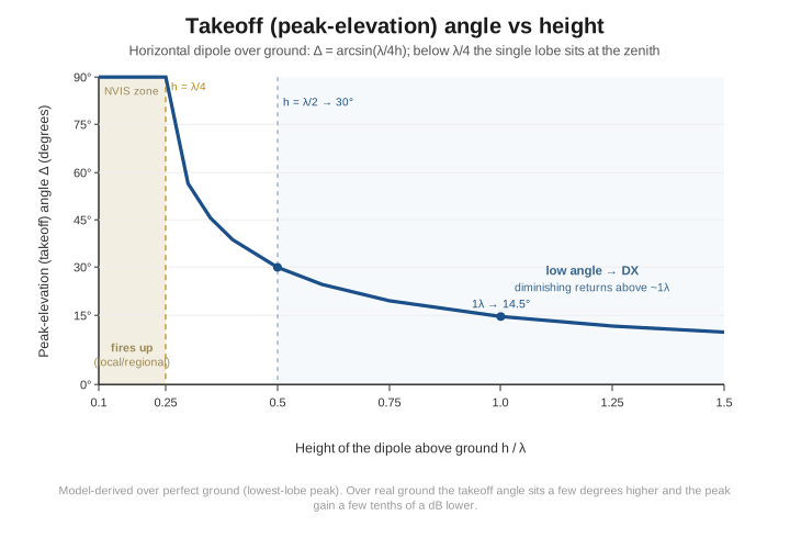
Reading the curve gives the band-by-band hang-height answer. A dipole at h = λ/2 has a takeoff angle of about 30° — a good general-purpose compromise that covers regional and medium-distance work and reaches into DX. A dipole at h = 1λ drops the main lobe to about 14.5°, squarely in the low-angle DX window, and adds a second, higher-angle lobe (~49°) that keeps regional paths alive too. Past about a wavelength the returns diminish: going from 1λ to 1.5λ only moves the takeoff angle from ~14.5° to ~9.6°, a few degrees for a 50% increase in tower height, and the peak gain barely changes. The practical rule the curve encodes is “λ/2 and up for DX, with the sweet spot around a wavelength, and little reason to chase height much beyond that.” On the low bands this rule collides with physics — a half-wavelength up on 80 m is ~40 m of mast and on 160 m it is ~80 m, heights almost no amateur achieves — which is precisely why low-band dipoles are usually de facto high-angle (NVIS-ish) antennas whether their owners intend it or not, and why the low bands lean on verticals and on accepting regional rather than DX coverage. On the high bands the rule is easy: a 20 m dipole at 10 m is already 0.5λ up, and at 20 m it is 1λ up and a genuine DX antenna.

Two real-ground caveats keep this honest. First, the arcsin(λ/4h) angles are the perfect-ground values; over real, lossy ground the takeoff angle of the lowest lobe sits a few degrees higher than the formula predicts, and the lobe is a little less sharply defined. Second, ground quality matters for the gain, not just the angle: the lobe-peak gain is a few tenths of a dB below the perfect-ground ideal over average soil and noticeably better over highly conductive ground such as salt water or a marsh — the well-known reason a seaside or salt-flat location is a DX advantage. The takeoff-angle curve tells you where to put your energy in elevation; the soil under the antenna tells you how much of it survives the reflection. Neither changes the headline guidance: for DX, get a horizontal dipole at least a half-wavelength up and ideally near a wavelength; beyond that, spend the effort elsewhere.

3.7 NVIS — the deliberately low dipole

The takeoff-angle curve has a regime that looks like a mistake and is in fact a tool: the very low dipole, h ≈ 0.1–0.2λ, whose single broad lobe fires nearly straight up. That is Near-Vertical Incidence Skywave (NVIS), and it is the right antenna for a specific and valuable job. A signal launched at a near-vertical angle on the lower HF bands strikes the ionosphere almost head-on, reflects back down, and returns to earth spread over a roughly circular footprint 0 to about 400 km in radius around the station — filling in the dreaded skip zone, the dead region between the limit of useful ground-wave (a few tens of km) and the closest distance that conventional low-angle skywave can reach (often 500–1500 km, depending on band and conditions). Where a high antenna optimised for DX leaves a doughnut of stations too close to work via skywave and too far to reach by ground-wave, the NVIS dipole blankets exactly that region with a strong, uniform signal.

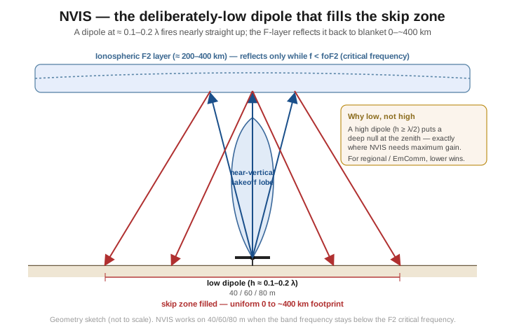
The geometry is the whole argument for hanging the antenna low. From Section 5, a dipole below λ/4 has its maximum at the zenith, and one around 0.15λ has a broad, strong near-vertical lobe — exactly matched to the near-vertical angles NVIS uses. A high dipole does the opposite: at h = λ/2 the array factor puts a deep null at the zenith, so a “good DX height” antenna is nearly blind in the one direction NVIS needs. This is the rare and instructive case where lower is better, and it directly contradicts the otherwise-sound “higher is better” instinct of Section 6 — the instinct is right for DX and wrong for regional coverage. A 40 m dipole at 5 m is a far better regional antenna than the same dipole at 15 m.

NVIS is the right tool when the mission is regional or emergency communications — a statewide net, disaster-relief traffic across a damaged region, agricultural or expedition comms across a few hundred km where there is no infrastructure and the distance is too far for VHF line-of-sight and too near for HF DX. It lives on 40, 60, and 80 m (and 160 m), because the physics demands a band whose frequency is below the ionosphere’s critical frequency foF2 — the highest frequency the F2 layer will reflect straight back at vertical incidence. foF2 rises with daytime ionization and falls at night, so the workable NVIS band shifts with the clock: 60 m and 40 m are the daytime NVIS workhorses, while 80 m (and sometimes 160 m) take over at night as foF2 drops below the 40 m frequency. When the band you are on is above foF2, the near-vertical signal punches through the layer into space instead of reflecting, and NVIS simply fails — the operational skill is choosing the band against the time of day and the solar conditions. The detailed propagation physics belongs to the hub’s propagation material; what this volume owns is the antenna half: hang it low, accept the high-angle pattern as a feature, and match the band to foF2.

3.8 Bandwidth and the SWR curve

Vol 2 established the feedpoint impedance at and around resonance as a function of length and height; this section lets frequency vary and watches the SWR trace out the antenna’s usable bandwidth. The driving physics is that a half-wave dipole is, near resonance, a series-resonant circuit — the radiation resistance is the loss term, and the element stores reactive energy that swings the feedpoint inductive above resonance and capacitive below it, exactly as Vol 1 described. As you move off the resonant frequency, the reactance grows roughly linearly with the detuning, the impedance walks away from the resistive value, and the SWR on the 50 Ω line climbs. Plotted against frequency the result is the characteristic V-shaped (or U-shaped) SWR curve with a sharp minimum at resonance.

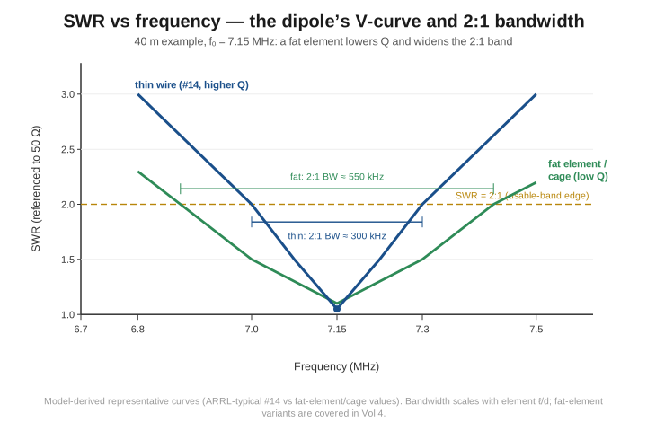
What sets the width of that V is the rate at which the reactance changes with frequency, and that rate is the element’s Q — the ratio of stored reactive energy to radiated power per cycle. A high-Q element has reactance that climbs steeply away from resonance, so the SWR shoots up over a narrow span; a low-Q element has reactance that changes gently, so the SWR stays low over a wider span. Making the criterion precise: feeding the resonant resistance R with a matched line, the SWR reaches 2:1 when the reactance magnitude reaches |X| = 0.707·R (the algebra: |Γ| = 1/3 at SWR 2, and |Γ|² = X²/(4R² + X²) = 1/9 solves to |X| = R/√2). The 2:1 bandwidth is simply the frequency span between the two points where the rising reactance crosses ±0.707·R, and it is inversely proportional to Q: wider bandwidth means lower Q.

The lever that sets Q for a wire dipole is the element’s length-to-diameter ratio ℓ/d — the same parameter that set the trim factor k in Vol 1. A fat element (low ℓ/d) stores less reactive energy per unit radiation, has a lower Q, and so has a wider bandwidth; a thin element (high ℓ/d) is higher-Q and narrower. This produces a counter-intuitive but real band-by-band pattern for the same #14 wire: on the low bands the wire is long, ℓ/d is enormous, Q is high, and the fractional bandwidth is narrow; on the high bands the wire is short, ℓ/d is much smaller, Q is lower, and the fractional bandwidth is wide. Representative 2:1-SWR bandwidths for a thin-wire (#14) dipole at typical heights are:

Table 1 — The lever that sets Q for a wire dipole is the element's length-to-diameter ratio ℓ/d — the same parameter that set the trim factor k in [Vol 1](/single-band-dipoles/vol-1/). A fat element (low ℓ/d) stores less reactive energy per unit radiation, has a lower Q, and so has a wider bandwidth; a thin element (high ℓ/d) is higher-Q and narrower. This produces a counter-intuitive but real band-by-band pattern for the same #14 wire: on the low bands the wire is long, ℓ/d is enormous, Q is high, and the fractional bandwidth is narrow; on the high bands the wire is short, ℓ/d is much smaller, Q is lower, and the fractional bandwidth is wide. Representative 2:1-SWR bandwidths for a thin-wire (#14) dipole at typical heights are

Band	Design freq (MHz)	2:1-SWR bandwidth (#14 wire)	Coverage
80 m	3.650	~120–180 kHz	only about a third of the 3.5–4.0 MHz band
40 m	7.150	~250–350 kHz	the full 7.0–7.3 MHz band
20 m	14.175	~600–800 kHz	well over the 350 kHz band
10 m	28.500	~1.5–2.0 MHz	the full band easily

The headline trap is 80 m: a single thin-wire dipole cut at band-centre covers only about a third of the band at SWR < 2:1, so it forces a choice — cut for the CW segment or the phone segment and tune across to the other, or widen the element. Widening the element is the standard cure, and it is exactly the low-Q move above: a fat element (tubing, or a wire dipole built physically thicker) flattens the V and widens the 2:1 band — the figure above shows a fat element taking a 40 m dipole from ~300 kHz to ~550 kHz — and a cage dipole (several parallel wires on spreaders, behaving as one very fat conductor) widens it further still. Those fat-element and cage variants, and the multi-resonant fan and folded approaches that cover more of a wide band, are the subject of Vol 4; the point this volume establishes is why they work — they lower the element Q — and what the thin-wire baseline they improve on actually delivers. The shape of the curve carries one more diagnostic worth knowing: a clean dipole’s SWR minimum should be a single sharp V at the design frequency, and anomalous extra dips or a minimum that shifts when you flex the feedline are the fingerprint of common-mode current making the coax part of the antenna — the Vol 2 balun problem showing up on the sweep rather than as RF in the shack.

3.9 Trim sensitivity — kHz per centimetre by band

The SWR curve’s sharp minimum sits at the resonant frequency, and the practical question the build procedure has to answer is how far that minimum moves when you change the element length — because the universal tuning method is to cut the wire a little long and trim it onto frequency. Since the resonant frequency is inversely proportional to length (f ∝ 1/L), a small fractional change in length produces an equal and opposite fractional change in frequency: Δf/f ≈ −ΔL/L. Rearranging to the form a builder uses — how many centimetres of wire per kilohertz of frequency shift — the sensitivity is ΔL/Δf ≈ L/f, and because L itself scales as 1/f, the length-per-kilohertz figure scales as 1/f². Trimming gets dramatically more delicate as you go up in frequency: a kilohertz of correction takes about half a centimetre of trim per side on 80 m but only a fraction of a millimetre on the high bands.

Representative trim sensitivities for a #14-wire dipole, expressed as the length removed from each end per kilohertz of upward resonance shift (trimming both ends equally), are:

Table 2 — Representative trim sensitivities for a #14-wire dipole, expressed as the length removed from each end per kilohertz of upward resonance shift (trimming both ends equally), are

Band	Trim per side per kHz of upward shift
80 m	~0.53 cm/kHz
40 m	~0.14 cm/kHz
30 m	~0.070 cm/kHz
20 m	~0.036 cm/kHz
15 m	~0.016 cm/kHz
10 m	~0.0088 cm/kHz
6 m	~0.0028 cm/kHz
2 m	~0.0003 cm/kHz (file, not cutters)

The 1/f² scaling is visible across the table — 80 m to 40 m is a factor of ~3.9, matching the (7.15/3.65)² ≈ 3.8 the frequency ratio predicts — and it carries two pieces of practical wisdom. First, trim small and trim symmetrically: on the high bands a careless “snip a few inches and re-sweep” overshoots wildly, and asymmetric trimming shifts the current maximum off the geometric centre and degrades the figure-8 pattern even though the SWR still bottoms out. Second, the sensitivity sets the headroom you cut into a fresh element — enough extra length to trim down onto frequency without ever having to add wire back (the cut-long rule of Vol 1, since a splice in a radiating element is a headache). The full cut-long-hoist-sweep-trim loop, the NanoVNA workflow that reads f_res off the SWR minimum, and the per-band headroom recommendations are the subject of Vol 5; what this volume contributes is the number — the kHz-per-centimetre sensitivity and its 1/f² scaling — that makes the loop converge in two or three iterations instead of a frustrated afternoon.

3.10 Where this volume hands off

This volume took the energy past the feedpoint and answered the two questions that decide whether a dipole works for you. On the pattern side: the free-space donut and the cos((π/2)cosθ)/sinθ factor it spins from (cited from Vol 1), the figure-8 with its ~78° half-power beamwidth and its end nulls (deep in free space, ~15–20 dB over ground), the linear polarization that matters ~20 dB on line-of-sight paths and far less on scrambled HF skywave, and — the dominant real-world effect — the ground-reflection lobing that turns the free-space elevation circle into lobes, lifts the lobe-peak gain ~6 dB toward the ~7.8 dBi quoted near h = λ/2, and sets a takeoff angle that falls as arcsin(λ/4h) so that DX wants λ/2-and-up while NVIS wants a deliberately low antenna firing into the zenith. On the frequency side: the V-shaped SWR curve, the element-Q-set 2:1 bandwidth (narrow on 80 m, wide on 10 m, widened deliberately by fat and cage elements), and the 1/f² trim sensitivity that the tuning loop has to respect.

The single-band dipole story continues. Vol 4 takes the clean reference geometry whose pattern, polarization, and bandwidth this volume established and bends it into deployable variants — the folded dipole (the wide-bandwidth, low-Q element this volume kept forward-referencing), the inverted-V (single-support, pattern broadened, nulls filled), the sloper (pattern skewed, a vertical-polarization component added), and the vertical dipole (the figure-8/circle assignment swapped for omnidirectional azimuth and vertical polarization) — and shows how each moves the pattern and bandwidth numbers anchored here. Vol 5 puts it on a rope: the step-by-step build, the cut-long-and-trim tuning loop with a NanoVNA that turns this volume’s trim-sensitivity table into an on-frequency antenna, the commercial-buy survey, and weatherproof deployment. The broader propagation physics — ionospheric layers, foF2 and the MUF, hop geometry — that decides when a given takeoff angle reaches a given distance lives in the hub’s propagation material, which this volume points to rather than reproduces.

3.11 Resources

• ARRL Antenna Book (25th+ ed.), the dipole/inverted-V and HF-antenna-and-the-earth chapters — the canonical amateur reference; reproduces the horizontal-dipole elevation-pattern-versus-height plots, the takeoff-angle and gain-versus-height curves, and the 2:1-bandwidth-by-band data used here.
• Balanis, Antenna Theory: Analysis and Design (4th ed.) — the academic derivation of the half-wave pattern factor, the 1.64/2.15 dBi directivity, the half-power beamwidth, and the image-theory treatment of an antenna over a ground plane.
• Stutzman & Thiele, Antenna Theory and Design (3rd ed.) — complementary treatment of the dipole pattern integral, beamwidth, and the array-factor approach to ground reflection.
• Kraus, Antennas — the classic development of the dipole far-field pattern and the ground-image array factor.
• ARRL / NVIS literature (e.g. the ARRL Antenna Book NVIS section and the standard NVIS field references) — the defensible source for the near-vertical-incidence geometry, the ~0.1–0.2 λ optimal-height guidance, and the foF2-versus-band operating window.
• L. B. Cebik (W4RNL) antenna-modeling papers — the deepest amateur-literature treatment of dipole-over-ground patterns, takeoff angle, and the real-ground-versus-perfect-ground deltas, archived across the antenna-modeling community.