The Wilkinson, and the Resistor That Dissipates Nothing

---

2.1 About this volume

Vol 1 established that a three-port splitter has to surrender one of {matched, lossless, isolated}, and that the Wilkinson surrenders losslessness in a purely formal way — it contains a resistor, so the theorem is satisfied, but that resistor carries no current when the outputs are behaving. This volume is the working-out of that sentence.

The Wilkinson is worth a volume because it is the only splitter most engineers will ever specify, because the derivation is genuinely short once the right decomposition is used, and because the seed chapter’s account of it contains three separate errors of mechanism sitting behind conclusions that are broadly right. Getting the mechanism straight is what lets a reader answer questions the chapter never asked: what happens if the substrate changes, what the second section costs, why the eight-way part in the catalogue does not look like Wilkinson’s eight-way divider.

Three results in this volume are worth stating at the top.

The first is that “bandwidth” as a bare percentage is not a specification. The seed gives the two-way Wilkinson a bandwidth of “~25 %” with nothing attached. Computed against a stated threshold, the same ideal network is 64.3 % wide at 15 dB, 36.1 % at 20 dB, 20.2 % at 25 dB and 11.3 % at 30 dB. All four are true. Which one is quoted is a marketing decision unless the threshold is given — and §5 finds that Wilkinson’s own 1960 abstract, which claims “about a 20 per cent band”, corresponds almost exactly to the 25 dB line.

The second is that the second section buys far more than the seed credits. Its §10.2 gives a three-section Wilkinson a bandwidth of 80 %. A two-section design computed here reaches 109.6 % at 20 dB, and three sections reach 125.0 % — a 4.33:1 frequency ratio. The chapter understates the technique it is recommending.

The third is that the chapter’s N-way table and its own four-way build describe different machines, and the build is the one that is right. §7 works out why, and the answer is a number: the sixteen-way star the table implies needs a 0.049 mm microstrip trace.

2.2 The even and odd modes, and why the derivation is one line

The Wilkinson is symmetric about the plane running between its two output ports. Any excitation of a symmetric network decomposes into a part that is symmetric about that plane — the even mode — and a part that is antisymmetric — the odd mode. Because the network is linear, the two modes can be analysed separately and added back together, and each one turns out to be trivial.

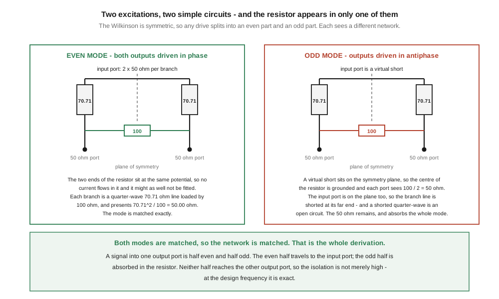
In the even mode, both output ports are driven with the same signal. The two halves of the network are doing identical things, so the two ends of the bridging resistor sit at identical potentials and no current flows through it. The resistor is invisible. What remains is a quarter-wave line of characteristic impedance Z₀√2 terminated, at the input end, by the input port’s 50 Ω seen as 2Z₀ = 100 Ω per branch — because in this mode the two branches share the input port’s resistance between them. A quarter-wave line transforms as Z_in = Z_line²/Z_load:

Z_in = 70.71² / 100 = 50.00 Ω

The even mode is matched exactly.

In the odd mode, the two output ports are driven in antiphase. Everything on the symmetry plane sits at zero potential — a virtual short. Two things follow. The centre of the bridging resistor is grounded, so each output port sees half of it, 100/2 = 50 Ω, straight to ground. And the input port is also on the symmetry plane, so the branch line is shorted at its far end; a quarter-wave of shorted line is an open circuit and contributes nothing in parallel. What each output port sees in the odd mode is therefore 50 Ω, and only 50 Ω:

Z_in = 50.00 Ω

The odd mode is matched exactly too.

Both modes matched means the output ports are matched, since any real excitation is a sum of the two. And the isolation follows immediately, which is the elegant part. A signal injected into output port 2 alone is, by definition, half even and half odd. The even half travels down both branches to the input port. The odd half is absorbed entirely in the resistor. Neither half arrives at output port 3 — the even and odd contributions at port 3 are equal in magnitude and opposite in sign, and they cancel exactly. The isolation of an ideal Wilkinson at its design frequency is not merely high; it is infinite.

That is the whole derivation, and it is why Vol 1 flagged the seed’s §4.2 admission — “the impedance match math is more complex than this simplified explanation captures” — as an honest sentence in the wrong place. The mathematics is four lines of quarter-wave transforms. What the chapter was missing was not sophistication but the decomposition, and without it the network genuinely does look intractable, because an analysis that tries to treat the resistor as an ordinary circuit element in a single-ended calculation has to carry a component whose current is zero by a symmetry it has not noticed.

2.3 70.71 and 100 arrive by two independent routes

The seed states that the branch impedance is “sqrt(50 × 100) = 70.7 Ω — the geometric mean of the input (50 Ω) and the bridging resistor (100 Ω)”. Both numbers in that sentence are correct and the relationship between them is not.

The branch impedance is set by the even mode, which does not contain the resistor at all. Two branches in parallel must present Z₀ at the input node, so each must present 2Z₀ = 100 Ω, and a quarter-wave line transforming 50 Ω into 100 Ω needs Z_line = √(50 × 100) = 70.71 Ω. The geometric mean is real, but it is the geometric mean of the load and twice the system impedance, and the 100 in it is 2Z₀, not the resistor.

The resistor is set by the odd mode, which does not contain the branch impedance in any binding way. Each output port must see Z₀ in the odd mode, and what it sees is half the resistor, so R/2 = Z₀ and R = 2Z₀ = 100 Ω.

Two derivations, two different modes, two different physical requirements — and both land on 2Z₀ because 2Z₀ is what “two of these in parallel must make one of those” means in both directions. That the same number appears twice is a consequence of the factor of two in “two-way”, not a relationship between the line and the resistor.

The distinction is not academic, and the test is what happens when the design changes. Build an unequal-split Wilkinson, dividing power in a ratio K² : 1 rather than 1:1, and the two quantities immediately part company: the branch impedances become Z₀√(K(1+K²)) and Z₀√((1+K²)/K³), which are different from each other, while the isolation resistor becomes Z₀(K + 1/K). At K = 1 all three collapse to 70.71, 70.71 and 100. At any other ratio the “geometric mean” story gives no guidance at all, while the mode analysis gives the answer directly. A mechanism that only works for the symmetric case is not a mechanism; it is a mnemonic that happens to be true once.

2.4 Where the loss actually is

The seed attributes the Wilkinson’s excess loss to the resistor: “3 dB inherent + ~0.3–0.5 dB resistive = ~3.5 dB per output”. The magnitude is realistic for a real part and should not be changed. The attribution is wrong, and §2 is why: in a balanced split the resistor carries no current, and a component carrying no current dissipates no power. The resistor’s contribution to the insertion loss of a correctly-operating two-way Wilkinson is exactly zero.

The excess loss is conductor loss and dielectric loss in the quarter-wave branch lines, plus connector and solder-joint resistance. That matters for three reasons, each of which is a prediction the chapter’s version cannot make.

It scales with the length of line, so it scales with the number of sections. §6’s three-section design has three times as much transmission line in each branch as the single-section design does, and therefore roughly three times the excess loss. Bandwidth in a Wilkinson is bought with copper, and the currency is decibels.

It depends strongly on the substrate. FR-4 has a dissipation factor around 0.02 at RF, which is poor; PTFE-based laminates are an order of magnitude better. A design that measures 0.3 dB of excess on Rogers may measure well over 1 dB on FR-4 at the same frequency, with no change whatever to the topology. The chapter’s own §14.1 offers “FR-4 (or Rogers RO4003 for low-loss)” as a substrate choice without saying what it changes; this is what it changes.

And it rises with frequency, roughly as √f for conductor loss and linearly for dielectric loss, whereas a resistor’s dissipation would not. A 0.3 dB excess measured at 500 MHz is not a 0.3 dB excess at 3 GHz.

There is one condition under which the resistor does dissipate, and Vol 1 §6 quantified it: whenever the two outputs are not identical. An output port terminated in something other than 50 Ω, or left open, or shorted, unbalances the split and generates an odd-mode component that lands entirely in the resistor. This is the answer to a question the chapter does not ask but every builder eventually does — what happens if one output of a splitter is left unterminated? The answer is that the input match degrades, the surviving output loses level, and the difference goes into a resistor that was sized on the assumption that it would never see any. Terminate unused ports.

2.5 Bandwidth is a number and a threshold

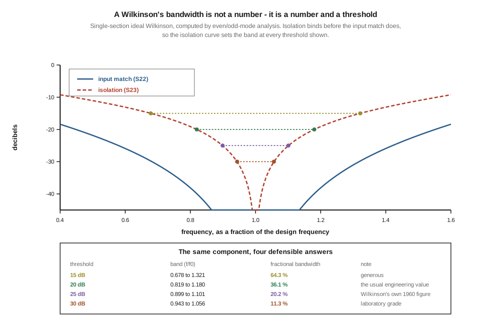
The seed gives the single-section two-way Wilkinson a bandwidth of “~25 % (typical 2-way design)”. No threshold is attached, and without one the figure cannot be checked, compared or used.

Computing the ideal network by the even/odd analysis of §2 and sweeping frequency gives the following, where the band is the range over which both the input match and the isolation are better than the stated figure:

Table 1 — Computing the ideal network by the even/odd analysis of §2 and sweeping frequency gives the following, where the band is the range over which both the input match and the isolation are better than the stated figure

threshold	band (f/f₀)	fractional bandwidth	ratio
15 dB	0.678 to 1.321	64.3 %	1.95:1
20 dB	0.819 to 1.180	36.1 %	1.44:1
25 dB	0.899 to 1.101	20.2 %	1.22:1
30 dB	0.943 to 1.056	11.3 %	1.12:1

Every row describes the same component. A catalogue entitled to choose its own threshold can describe this divider as a 64 % device or an 11 % device without saying anything false.

Two observations make the table more useful than a caution against marketing.

The isolation binds, not the match. At every threshold in the table the isolation curve reaches the limit first; the input match is still comfortably better. That is a design fact worth carrying: if an application genuinely does not need isolation — two instruments that emit nothing, in Vol 1 §7’s framing — a single-section Wilkinson will hold a good input match far outside its nominal band, and the “bandwidth” in the catalogue is not the constraint being violated.

And the 25 dB row is Wilkinson’s own. His 1960 paper describes his divider as providing “isolation between output terminals and approximately matched terminal impedances over about a 20 per cent band”. The computed 25 dB figure is 20.2 %. That is close enough to be the same claim, which means the seed’s 25 % is not invented — it is a real number that has lost its threshold somewhere between 1960 and the chapter. The seed’s figure is confirmed, not corrected; what is added is the missing variable.

That distinction matters, because this is now the third occurrence of the same defect class in this hub. The antenna-tuners dive found a loss table indexed against SWR when the binding variable was the load impedance, and two feedline tables that omitted the frequency. The transmitting-loops dive found a bandwidth column carrying half-power figures under a 2:1-SWR heading. Here a bandwidth is quoted with no threshold at all. In none of the three cases was the number fabricated. In all three the number was correct for one unstated condition and wrong everywhere else, which is a subtler failure than invention and considerably harder to catch by reading.

2.6 What a second section buys

The way to widen a Wilkinson is to replace the single quarter-wave transformer in each branch with a cascade of them, stepping the impedance from Z₀ up to 2Z₀ in stages, and to fit an isolation resistor at each junction rather than only at the output end. The even mode then sees a multi-section impedance transformer, whose bandwidth behaviour is classical; the odd mode sees a cascade of shorted stubs loaded by the resistors.

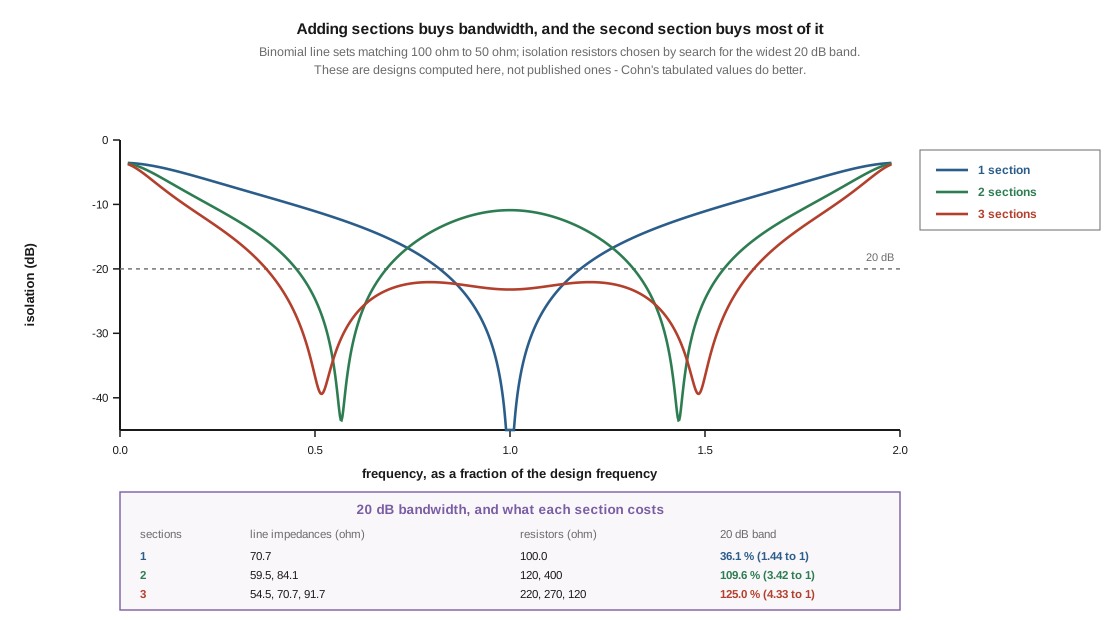
Computed here on binomial line sets, with resistor values found by a coarse search for the widest 20 dB band:

Table 2 — Computed here on binomial line sets, with resistor values found by a coarse search for the widest 20 dB band

sections	branch line impedances (Ω)	isolation resistors (Ω)	20 dB band	ratio
1	70.71	100	36.1 %	1.44:1
2	59.46, 84.09	120, 400	109.6 %	3.42:1
3	54.53, 70.71, 91.70	220, 270, 120	125.0 %	4.33:1

Against this, the seed’s §10.2 gives a three-section Wilkinson a bandwidth of 80 %, which understates it substantially — a two-section design already beats that figure. The chapter is underselling the technique it recommends.

Three honest limits belong with this table.

These are designs computed here, not published ones. The line impedances are binomial, which is a standard and defensible choice, but the resistor values came from a search over a coarse grid conducted for this volume. Seymour Cohn’s 1968 paper on the class gives tabulated values derived properly, and those will do better than a grid search. The numbers above should be read as a demonstration of what the topology can reach, not as a design to be built from.

The 25 dB row is missing on purpose. Neither the two-section nor the three-section design found here meets 25 dB across any contiguous band, because the binomial line set combined with grid-chosen resistors leaves ripple that crosses the line. That is a limitation of the design method used here rather than of multi-section Wilkinsons, and it is recorded rather than hidden.

And the third section is nearly all diminishing return. Going from one section to two adds 73.5 percentage points of bandwidth; going from two to three adds 15.4 more, for another third of a wavelength of line in each branch and another pair of resistors. Combined with §4’s finding that excess loss scales with line length, the two-section design is the one that earns its keep, and that is the practical conclusion of this section.

2.7 N ways: the star, the tree, and a chapter that contradicts itself

Wilkinson’s original paper describes a circularly symmetric divider: N branch lines meeting at a common input node, each of impedance Z₀√N, with resistors running from each output to a common floating star point. The seed reproduces the impedance scaling correctly, and it should be confirmed rather than questioned — Z₀√N gives 70.7, 86.6, 100, 141.4 and 200 Ω for N of 2, 3, 4, 8 and 16, which is exactly the chapter’s table. Its insertion-loss column is also sound: the figures sit about 0.5 dB above the inherent 10·log₁₀(N), which is a fair allowance.

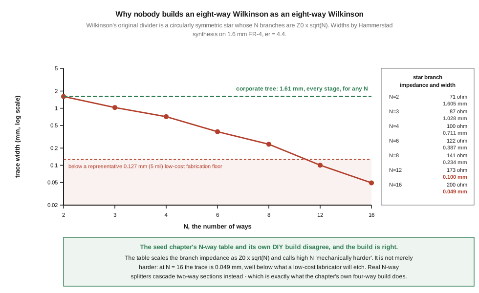
What the chapter then says is that higher N “becomes mechanically harder to realize (high-Z lines need very thin conductors or wide separation)”. That is true and it is a serious understatement. Synthesising the required microstrip on 1.6 mm FR-4:

Table 3 — What the chapter then says is that higher N "becomes mechanically harder to realize (high-Z lines need very thin conductors or wide separation)". That is true and it is a serious understatement. Synthesising the required microstrip on 1.6 mm FR-4

N	branch impedance	microstrip width on 1.6 mm FR-4
2	70.7 Ω	1.605 mm
4	100.0 Ω	0.711 mm
8	141.4 Ω	0.234 mm
16	200.0 Ω	0.049 mm

A 0.049 mm trace is about two thousandths of an inch. It is not merely hard; it is below what a low-cost fabricator will etch at all, and it would have unusable current-handling and enormous conductor loss if it could be made. The star topology does not scale, and the reason it does not is quantitative.

The answer real hardware uses is the corporate tree: cascade two-way dividers, each identical, in a binary structure. A four-way is two stages of two-way; an eight-way is three stages. Every line in the structure is 70.71 Ω, every resistor is 100 Ω, and the trace width stays at 1.605 mm no matter how large N becomes. The inherent loss is the same 10·log₁₀(N) — the tree cannot beat physics — but the excess loss accumulates as the number of stages, log₂N, rather than exploding.

And the chapter already knows this. Its §15.2, describing the four-way HF build, says in as many words: “The 4-way ferrite-core splitter uses a two-stage Wilkinson architecture: Stage 1: input → two outputs; Stage 2: each of those two outputs → two more outputs.” That is a corporate tree, correctly described, four sections after a table that implies a four-way is a single star with 100 Ω branches. Both descriptions are in the same chapter and they are different machines. The build is right and the table’s framing is what needs the correction — which is the same shape as the defect the antenna-tuners dive found, where the correct statement sat in plain language between two drawings that contradicted it.

One consequence of the tree is worth stating because it is a trap. In a corporate tree the isolation between two outputs depends on how far apart they are in the tree. Two outputs sharing a final-stage divider are isolated by that divider alone. Two outputs on opposite halves of an eight-way are isolated by three cascaded stages, and are far better isolated. A single “isolation” figure on an N-way datasheet is therefore a worst case across port pairs, and the worst case is always the adjacent pair.

2.8 When a quarter wave is forty metres

Everything above assumes a quarter-wave transmission line is a practical object. At 1 GHz on FR-4 it is 42 mm and the assumption is safe. At 3.5 MHz it is about 21 metres of coaxial cable, and it is not.

That single fact governs the whole of HF distribution, and it is why the splitters in an HF station are built from ferrite-cored transmission-line transformers rather than from quarter-wave sections. The devices are still Wilkinson dividers in topology — an in-phase power split with an isolation resistor bridging the outputs — but the quarter-wave impedance transformer is replaced by a wound transformer, which achieves the same impedance ratio by turns ratio rather than by electrical length, and is therefore broadband rather than resonant. The BALUNs and UNUNs dive covers the transformer technology itself in depth; what matters here is the two things the substitution changes.

The bandwidth becomes a ratio rather than a percentage, and it is enormous. A quarter-wave Wilkinson is a resonant structure with a band centred on one frequency. A transformer splitter is bounded below by the magnetising inductance of its primary — at some frequency the winding’s reactance stops being large compared with 50 Ω and starts shunting the signal away — and bounded above by leakage inductance and interwinding capacitance. Between those limits it is flat. Decade-wide parts are ordinary, and the seed’s “10:1 or wider” is correct.

And the isolation resistor is still 2Z₀. The seed’s §7.1 says the ferrite splitter uses “50 Ω terminations at the bridging resistor location (similar to Wilkinson’s 100 Ω)”, which is wrong twice: it is 100 Ω, not 50, and the parenthesis concedes the right answer while stating the wrong one. The odd-mode argument of §2 does not care whether the impedance transformation was done by a quarter-wave line or by a winding. Each output port must see Z₀ in the odd mode, it sees half the bridging resistor, and therefore the bridging resistor is 2Z₀ = 100 Ω. Every commercial two-way transformer splitter uses 100 Ω for this reason.

The seed also explains the transformer splitter’s slightly poorer isolation — it gives 18–25 dB against the Wilkinson’s 20–25 — by saying “the ferrite has less ideal impedance behaviour”. The observation is right and the mechanism is vague. Isolation in either topology fails through imbalance: it is exact only when the two halves of the network are identical. A quarter-wave Wilkinson etched on a symmetric board is very nearly identical by construction. A wound transformer’s two halves differ by whatever the winding tolerance, core inhomogeneity and lead-dress differences amount to, and that residual asymmetry leaks even-mode energy into the odd-mode path. The limit is mechanical symmetry, not the permeability of the ferrite, which is why hand-wound splitters improve markedly when the two windings are made from a single bifilar pair rather than wound separately.

One warning about the seed’s HF product list belongs here, although the survey itself is Vol 5’s job. Of the parts it names as HF transformer splitters, not one is an HF part. The Mini-Circuits ZN2PD2-50+ it lists at “0.5–50 MHz” is specified at 500–5000 MHz; the ZN4PD-642+ it lists at “0.5–50 MHz” is a 1600–6400 MHz part; the MECA 802-2-1.500V it lists at “1.5–1500 MHz” covers 0.8–2.2 GHz. Vol 5 works out how three rows went wrong the same way.

2.9 Where this volume hands off

The Wilkinson’s behaviour follows from one decomposition. In the even mode the resistor is invisible and each branch transforms 50 Ω to 100 Ω, so two branches in parallel match the input exactly. In the odd mode the symmetry plane is a virtual short, the branch line becomes a shorted quarter-wave and disappears, and each output sees half the resistor — which is why the resistor is 2Z₀, by a route entirely independent of the one that fixes the branch impedance at Z₀√2. Isolation is exact at the design frequency because the even and odd contributions at the far output cancel. The excess loss is in the copper and the dielectric, not the resistor, which is why it scales with sections and substrate rather than with resistor value. Bandwidth is 64.3 %, 36.1 %, 20.2 % or 11.3 % depending entirely on the threshold demanded, and Wilkinson’s own 20 % is the 25 dB figure. A second section nearly triples the 20 dB band; a third adds little. And beyond two ways the star gives way to the tree, for a reason that can be stated as a trace width.

From here:

• Vol 3 — Four ports, and what the phase buys takes the other escape from Vol 1’s theorem. A four-port can be lossless, reciprocal and matched at every port simultaneously, and the branch-line hybrid, the rat-race and the coupled-line coupler all are. The reward is that the phase relationship between the outputs becomes a design parameter; the price is a fourth port that must be terminated.
• Vol 4 — Sampling instead of splitting covers the deliberately unequal divider — the directional coupler — and the specification that governs it, which is directivity rather than coupling.
• Vol 5 — DIY build, measurement and buys builds a Wilkinson on FR-4 using §7’s synthesis, measures it, and surveys the market. The seed’s own build instructions place a 100 MHz design on a 90 × 60 mm board; §7’s numbers put the quarter-wave at 421 mm.

Every figure in this volume is from an idealised network with lossless lines and ideal lumped elements. No measurement here is first-hand.

2.10 Resources

• E. J. Wilkinson, An N-Way Hybrid Power Divider, IRE Trans. MTT, vol. 8, no. 1, pp. 116–118, 1960 — the original. Its “about a 20 per cent band” is the claim §5 reproduces independently and pins to a 25 dB threshold, and its circularly symmetric N-way is the star topology §7 shows does not scale.
• S. B. Cohn, A Class of Broadband Three-Port TEM-Mode Hybrids, IEEE Trans. MTT, 1968 — the multi-section extension, and the source of properly-derived resistor values. Cited here from its standard description in the literature rather than read first-hand; §6’s resistor values were computed independently and are not Cohn’s.
• D. M. Pozar, Microwave Engineering, 4th ed., §7.3 — the even/odd-mode analysis in its textbook form.
• E. Hammerstad and Ø. Jensen, Accurate Models for Microstrip Computer-Aided Design, IEEE MTT-S, 1980 — the microstrip synthesis behind §7’s widths and the quarter-wave lengths quoted throughout.
• BALUNs and UNUNs, Vol 2 — transmission-line transformer topology, the technology §8’s HF splitters are built from.
• Antenna tuners, Vol 3 — the first instance in this hub of the missing-variable defect §5 identifies here for the third time.
• Transmitting loops, Vol 2 — the second instance, where a half-power bandwidth was printed under a 2:1-SWR heading.