Transmitting Loops · Volume 2
Q, Bandwidth and the Capacitor
The bandwidth the previous edition doubled and its own section title overstated by forty, the femtofarads of tuning resolution nobody quotes, the capacitor voltage the chapter got right in one section and wrong in another, and the loop that heats itself off frequency in ninety seconds
2.1 About this volume
Vol 1 established what a small loop costs in efficiency and why. This volume is about the other consequence of the same high Q, and it is the one that decides whether you can live with the antenna: the bandwidth, the capacitor that sets it, and the voltage that capacitor has to stand.
All three are computable from the model in Vol 1 §3, and all three came out differently from the previous edition.
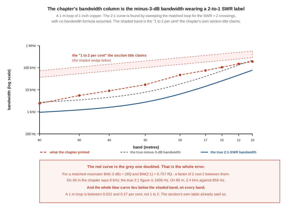
The bandwidth figures are the half-power bandwidth wearing a 2:1-SWR label. §2 derives the factor — 2√2 — and confirms it by sweeping the matched loop for the SWR = 2 crossings rather than trusting any formula. On 40 m the previous edition says 9 kHz; the true figure is 1.6 kHz.
And the section those figures live in is titled “the 1-2% reality” while its own table says 0.07 %. That is not a subtlety. A 1 m loop runs between 0.022 % and 0.27 % of centre frequency — fifteen to forty times narrower than its own headline, and the table printed directly beneath the headline already said so.
The capacitor voltage is the one that matters, and here the previous edition is right in one place and wrong in another. §3.3 states that “the 5–10 kV that develops across the capacitor at resonance under 100 W will arc air-variable capacitors” — which brackets the computed answer. §11 then calculates 2.3 kV for the same antenna at the same power, and builds its component-selection table on that. The section doing the calculating is itself titled “the 5 kV consideration”. §4 works out what the voltage really is and where it peaks, which is not where the previous edition looks.
And there is a mechanism the previous edition observes but never explains. It notes that a loop’s SWR drifts during operation and attributes it to temperature and humidity. §7 computes the actual cause: on 80 m the loop dissipates 98 of your 100 watts in its own tubing, which heats it at 0.16 K/s and walks it half a bandwidth off frequency in about ninety seconds of continuous carrier.
2.2 The bandwidth, and the label on it
A resonant circuit has two bandwidths that get confused, and on an antenna with a Q of three thousand the confusion is worth two and a half times.
The half-power bandwidth is where the delivered power falls to half — the −3 dB points. For a matched resonator that is
BW(−3 dB) = 2f / Q_unloaded
the factor of two arising because a matched resonator’s loaded Q is half its unloaded Q: the source resistance, referred into the circuit, equals the loss resistance.
The 2:1-SWR bandwidth is where the reflection coefficient reaches one third. Working it through for a matched series resonator gives
BW(2:1) = 0.7071 · f / Q_unloaded
a factor of 2√2 narrower. The lead figure plots both, and the 2:1 curve on it is not from that formula — it is found by sweeping the loop and locating the crossings, so the formula and the sweep are independent confirmations of each other.
For a 1 m loop of 1″ copper:
Table 1 — For a 1 m loop of 1″ copper
| band | Q_unloaded | previous edition | true −3 dB | true 2:1-SWR |
|---|---|---|---|---|
| 80 m | 2 701 | 2.4 kHz | 2.70 kHz | 956 Hz |
| 40 m | 3 147 | 9 kHz | 4.54 kHz | 1.61 kHz |
| 20 m | 1 559 | 47 kHz | 18.2 kHz | 6.43 kHz |
| 10 m | 260 | 190 kHz | 219 kHz | 77.6 kHz |
Look at the middle two columns. The previous edition’s figures track the −3 dB bandwidth closely on the bands where its Q values are close to right, and diverge where they are not. It computed the correct quantity and labelled it as the other one.
⚠ One thing it got right and should not be corrected. Its Q column — 1500 on 80 m, 800 on 40 m — is roughly the loaded Q, half the unloaded figure, and that is a legitimate way to quote a matched resonator. The error is entirely in what is done with it afterwards.
2.2.1 The section title
The section containing that table is headed “Frequency response & bandwidth — the 1-2% reality”, and 1–2 % is repeated in its opening line as “the defining property of a small magnetic loop”.
As a fraction of centre frequency, the true 2:1-SWR bandwidths are:
Table 2 — As a fraction of centre frequency, the true 2:1-SWR bandwidths are
| band | 80 m | 40 m | 20 m | 10 m |
|---|---|---|---|---|
fraction of f | 0.026 % | 0.022 % | 0.045 % | 0.272 % |
Between fifteen and forty times narrower than the headline, and never once inside it. The lead figure shades the 1–2 % region so the gap is visible: the true curve lies below it across the entire HF range.
What makes this worth more than a correction is that the section’s own table already refuted its own title. Its 80 m entry of 2.4 kHz is 0.066 % of 3.65 MHz. Anyone dividing one of its own numbers by one of its own frequencies would have caught it. The headline and the table were evidently written at different times and never reconciled — which is a failure mode worth watching for, because it leaves the correct information sitting in the document next to the wrong information.
2.3 The resolution nobody quotes
A 1.6 kHz bandwidth on 40 m is a number most operators can picture: about a quarter of an SSB channel. What is harder to picture is what it demands of the tuning mechanism.
Differentiating the resonance condition gives df/dC = −f/(2C), so for the 1 m loop:
Table 3 — Differentiating the resonance condition gives df/dC = −f/(2C), so for the 1 m loop
| band | C at resonance | one picofarad is worth | in bandwidths |
|---|---|---|---|
| 80 m | 806 pF | 2.3 kHz | 2.4 |
| 40 m | 210 pF | 17.0 kHz | 10.6 |
| 20 m | 53 pF | 133 kHz | 20.6 |
| 10 m | 13 pF | 1 077 kHz | 13.9 |
On 40 m, one picofarad moves the loop ten bandwidths off frequency. On 20 m, twenty.
Invert that and you get the specification the tuning drive actually has to meet.
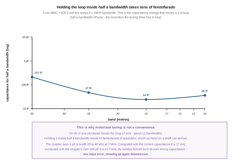
Table 4 — 3. The resolution nobody quotes
| band | capacitance for half a bandwidth |
|---|---|
| 80 m | 211 fF |
| 40 m | 47 fF |
| 20 m | 24 fF |
| 10 m | 36 fF |
Tens of femtofarads. That is a few thousandths of a degree of rotation on a typical air variable, and it is why every serious magnetic loop has a motor, a reduction gearbox and often a vernier stage — not as a convenience for reaching the antenna, but because the required resolution is beyond what a hand on a shaft can produce even standing next to it.
The previous edition gets to a similar practical conclusion by a different route, and it is worth noting that its number here is wrong in a way that is now familiar. It says “a capacitor that moves 1 pF shifts the resonance by 20–40 kHz at 7 MHz.” Computed with the correct capacitance the figure is 17 kHz; computed with the 165 pF its own §3.2 gives — which Vol 1 showed belongs to a 10 mm conductor rather than the 1″ tubing specified two paragraphs earlier — it is 21.7 kHz. Its sensitivity figure follows correctly from its own wrong capacitance. One input error, showing up again three sections downstream.
2.4 The capacitor voltage, and where it really peaks
This is the section with consequences for hardware.
The loop is a series resonant circuit, so at resonance the voltage across the capacitor is Q times the voltage across the whole circuit. Written directly:
V_cap = I · X_L, with I = √(P / R_total)
and the useful compact form is V_cap = √(P · Q_u · X_L).
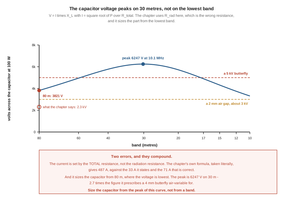
The previous edition writes it as V_cap = (√(P / R_rad)) × X_cap. R_rad is the wrong resistance — the current is set by the total resistance the transmitter drives, which is radiation plus loss, and on this antenna the loss is the larger part by far. The error’s direction is not subtle either: taken literally its own formula gives 487 A for a 1 m loop at 100 W on 80 m, against the 33 A the same paragraph states and the 70.7 A that is correct. The formula, the stated current and the truth are three different numbers.
Sweeping it properly:
Table 5 — Sweeping it properly
| band | 80 m | 60 m | 40 m | 30 m | 20 m | 15 m | 10 m |
|---|---|---|---|---|---|---|---|
V_cap at 100 W | 3 821 | 4 950 | 5 774 | 6 246 | 5 721 | 4 318 | 3 312 |
⭐⭐ The voltage peaks on 30 metres, and the previous edition sizes the capacitor from 80 metres. That is the finding of this volume with the most direct consequence for a build. V_cap = √(P·Q_u·X_L), and while Q_u falls as frequency rises, X_L rises faster over the lower half of the range — so the product peaks in the middle, around 10 MHz, not at the bottom.
Sizing the capacitor for the lowest band under-sizes it by 63 %.
2.4.1 The chapter already knew
What makes this more than an arithmetic slip is that the correct figure is in the same document.
§3.3, discussing why vacuum variables are worth their price, says: “The 5–10 kV that develops across the capacitor at resonance under 100 W will arc air-variable capacitors with insufficient plate spacing.”
5–10 kV. The computed range across the bands is 3.3–6.2 kV, so §3.3 is high but broadly right, and certainly right about the engineering consequence.
Then §11 — a section whose own title is “Power handling — capacitor voltage, the 5 kV consideration” — computes 2.3 kV, and its sizing table prescribes for that:
| 100 W | ~2.3 kV | Butterfly air-variable with 4 mm spacing, or vacuum-variable |
🔴 So the document contains the right answer in §3.3, a figure 2.7× lower in §11, a section title in §11 that agrees with §3.3 rather than with §11’s own body, and a component recommendation built on the lowest of the three. A builder following the table fits a part rated for less than half the peak voltage, and §11.2 — two subsections earlier — describes in detail what then happens: the arc carbonises the insulators, the SWR goes to infinity, and the amplifier’s protection trips.
This dive has now found the same shape in three chapters: the correct statement and its contradiction sitting in one document, with the wrong one driving the recommendation. It is why every number in this dive was computed rather than read.
2.5 Getting power in: the coupling loop
The capacitor sets the frequency. Something else has to get the power in, and on a circuit whose total resistance is twenty milliohms that is not a trivial job — you are matching 50 Ω to a load two and a half thousand times smaller.
The usual answer is a small coupling loop, typically about a fifth of the main loop’s diameter, mounted at the point of the main loop opposite the capacitor and fed directly from the coax. It works by mutual inductance, and the resistance the transmitter sees is
R_in = (ωM)² / R_total
where M is the mutual inductance between the two loops. Two separate adjustments therefore exist and the previous edition is right to separate them: the capacitor is resonance and the coupling loop is impedance, and they interact only weakly.
2.5.1 The ratio table
The previous edition gives a table of coupling ratios:
Table 6 — The previous edition gives a table of coupling ratios
| coupling / main diameter | 1/8 | 1/5 | 1/4 | 1/3 |
|---|---|---|---|---|
| feedpoint impedance | 12 Ω | 50 Ω | 80 Ω | 150 Ω |
Tested against a model, it is neither derived nor badly wrong. R_in goes as M², and for a small coupling loop sitting in a roughly uniform field M scales with its area — so a simple model predicts R_in ∝ d⁴. The table’s own implied exponent wanders between 2.1 and 3.0 from row to row, and the numbers track a d² law more closely than a d⁴ one, with the 1/8 row out of line even with that.
⚠ That is worth stating carefully rather than as a defect. A real coupling loop is not a uniform-field problem: it has its own inductance, its position and tilt matter, and the field it sits in is anything but uniform near the conductor. So d⁴ is a guide rather than a law, and the honest description of the table is that it is a plausible starting point, not a design tool — which matches practice, since every builder ends up adjusting the coupling loop empirically anyway. The 1/5 rule of thumb is sound; the three rows either side of it should not be trusted to a percentage.
2.5.2 What the table hides, and it matters more
The larger problem is what the table’s shape implies. Presented as a fixed geometric ratio giving a fixed impedance, it suggests the coupling loop is a set-and-forget part.
It is not, because R_in ∝ ω²/R_total and both of those change across HF. Setting a coupling loop for a perfect match on 40 m:
Table 7 — It is not, because Rin ∝ ω²/Rtotal and both of those change across HF. Setting a coupling loop for a perfect match on 40 m
| band | R_total | R_in | SWR |
|---|---|---|---|
| 80 m | 20.0 mΩ | 21.9 Ω | 2.28:1 |
| 60 m | 25.7 mΩ | 36.8 Ω | 1.36:1 |
| 40 m | 33.7 mΩ | 50.0 Ω | 1.00:1 |
| 30 m | 57.7 mΩ | 58.5 Ω | 1.17:1 |
| 20 m | 135 mΩ | 49.1 Ω | 1.02:1 |
| 15 m | 530 mΩ | 28.0 Ω | 1.79:1 |
| 10 m | 1 625 mΩ | 16.4 Ω | 3.04:1 |
⚠ The bottom two rows are past Vol 1’s validity limit and are indicative only.
⭐ A fixed coupling loop is good over about two octaves in the middle of the range and falls away at both ends — which is exactly the behaviour owners of commercial loops report, and it is a consequence of the formula rather than of anything being badly made. The rise and fall happen for different reasons at the two ends: at the low end ω² is small, at the high end R_total has grown by two orders of magnitude.
Three practical consequences follow:
- A loop that matches beautifully on its middle bands and shows 2.5:1 at the extremes is behaving correctly. Do not chase it with the capacitor; the capacitor sets frequency, not impedance.
- If you want a match everywhere, the coupling has to be adjustable too — which is why better designs make the coupling loop moveable or hinged rather than fixing it at a ratio.
- A modest mismatch here is cheap. Vol 1 showed the loop is throwing away most of the power in its own conductor regardless; a 2:1 at the feedpoint is a fraction of a decibel against that. Getting the coupling roughly right and leaving it is a defensible engineering choice, and it is what most commercial loops do.
2.6 Choosing the capacitor
With the real voltage curve in hand the component choice becomes straightforward, and mostly agrees with the previous edition’s conclusion even though it disagrees with its arithmetic.
Size for the peak of the curve, not for a band. For a 1 m loop at 100 W that means about 6.3 kV, and with any sane derating a 10 kV part. If the loop is only ever used on 80 m you can size for 3.8 kV — but almost nobody builds a single-band magnetic loop, because tuning range is the reason to build one at all.
Scale with the square root of power. V ∝ √P, so 400 W doubles the voltage rather than quadrupling it. A 1 m loop at the legal limit peaks near 24 kV, which is why kilowatt magnetic loops are rare, expensive and built around large vacuum variables.
The three families, with the previous edition’s own summary and where it needs qualifying:
Table 8 — The three families, with the previous edition's own summary and where it needs qualifying
| type | rating | note |
|---|---|---|
| Vacuum variable (Jennings, Comet) | 5–15 kV | The right answer above QRP. Sealed, and its loss is genuinely low |
| Butterfly air variable | 1–5 kV | Adequate at QRP and marginal at 100 W. ⚠ Its virtue is not the rating — it is that a butterfly has no wiper contact, so the RF current does not cross a rubbing joint |
| Plate air variable | 0.5–2 kV | Avoid for transmitting. The wiper is both a loss and a failure point |
⭐ That wiper point deserves more emphasis than the previous edition gives it. Vol 1 showed the whole antenna’s loss resistance is around twenty milliohms. A rubbing contact carrying seventy amps can easily contribute several milliohms — a double-digit percentage of the total — and unlike the tubing it will get worse with age and oxidation. The butterfly’s split-stator geometry, which puts the rotor in series with nothing, is a bigger deal on a magnetic loop than on any other antenna, because there is so little resistance for it to be measured against.
⚠ The previous edition contradicts itself on price and neither figure should be quoted without checking: §3.3 puts vacuum variables at “$400–1500 used”, while §15 says they are “available on the surplus market for $100–300.” Vol 5 owes a dated survey; until then, treat both as unverified.
2.7 The loop heats itself off frequency
The previous edition lists among its gotchas: “My loop’s SWR drifts during operation — true, and it’s the loop’s biggest annoyance. The capacitor’s plate spacing changes slightly with temperature, and the loop’s electrical length changes slightly with humidity.”
The observation is right and the explanation is not the main mechanism. The main mechanism is that the loop is heating itself, and it is heating itself with most of your transmitter’s output.
From Vol 1’s two resistances, at 100 W into a 1 m loop of 1″ copper:
Table 9 — From [Vol 1](/transmitting-loops/vol-1/)'s two resistances, at 100 W into a 1 m loop of 1″ copper
| band | radiated | into the copper |
|---|---|---|
| 80 m | 2.1 W | 97.9 W |
| 40 m | 18.5 W | 81.5 W |
| 30 m | 43.4 W | 56.6 W |
| 20 m | 71.3 W | 28.7 W |
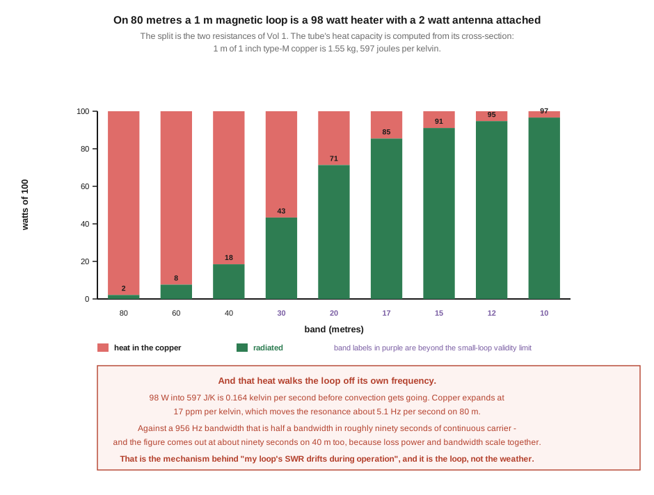
On 80 metres a 1 m magnetic loop is a 98 watt heater with a 2 watt antenna attached. That is not a criticism — Vol 1 §6 showed it still beats the alternatives available in the same space — but it has a consequence the previous edition misses.
One metre of 1″ type-M copper tube is about 1.55 kg, with a heat capacity near 597 J/K. Ninety-eight watts into that is 0.164 kelvin per second before convection gets going, and the first minute of a transmission is close to adiabatic. Copper expands at 17 ppm/K, which moves the loop’s inductance and therefore its resonance by roughly 5.1 Hz per second on 80 m.
Against a 956 Hz bandwidth, that is half a bandwidth in about ninety seconds of continuous carrier.
⭐ And the figure comes out at about ninety seconds on 40 m too — 8.3 Hz/s against a 1 606 Hz bandwidth — because the dissipated power and the bandwidth scale together as you change band. The drift time is close to a property of the antenna rather than of the band, which is a tidier and more useful statement than any per-band table.
So the practical picture is:
- On SSB with normal duty cycle, you will not notice much. The loop cools between overs.
- On a long key-down mode — RTTY, FT8 at high duty, a tuning carrier, AM — the loop walks off tune while you transmit, and an auto-tuning controller is not a luxury.
- The fix is thermal mass and surface area, not a better capacitor. Fatter tubing raises efficiency and heat capacity and cooling area, which is three reasons pointing the same way.
⚠ Two honest caveats. These are adiabatic figures; real convection reduces the steady-state rise substantially, so ninety seconds is a lower bound on the time to drift, not a prediction of a cliff. And the capacitor’s own temperature coefficient is a real additional term that this model does not include — the previous edition is not wrong that it exists, only about its relative size.
2.8 Where this volume hands off
The high Q that Vol 1 computed has three consequences and the previous edition mis-stated all of them. Its bandwidth figures are the half-power bandwidth, a factor of 2√2 wide of the 2:1-SWR bandwidth they claim to be, and the section holding them is titled with a figure its own table refutes by fifteen to forty times. The tuning resolution the antenna demands is tens of femtofarads, which is the real argument for a motor drive. The capacitor voltage peaks at 6.2 kV on 30 metres, not 2.3 kV on 80 — and the chapter’s own §3.3 and §11 title both said so while its §11 body and its component table did not. And the loop dissipates most of your power in its own tubing, which is what actually drifts it off frequency, in about ninety seconds of key-down on any band.
From here:
- Vol 3 — Full-wave loops leaves this family entirely. Delta, quad, square, cubical quad and hex beam are resonant current-element antennas with dipole-class bandwidth and dipole-class feedpoint impedance. Nothing in Vols 1 or 2 applies to them, and the previous edition’s decision to cover both under one heading is the main reason the two get confused.
- Vol 4 — Choosing, siting and operating takes pattern and practice, including a pattern claim that is inverted: a horizontal small loop nulls straight up, which is the opposite of what the previous edition says and undoes the NVIS recommendation built on it.
- Vol 5 — DIY build and buys builds a loop with the capacitor sized from §4’s curve rather than from a band, and surveys the market — where three of the products listed are from a manufacturer that stopped manufacturing in May 2024.
One item is owed and it is the same one Vol 1 owes: no measurement here is first-hand. The bandwidth and the voltage are both directly measurable — a VNA sweep gives the first in a minute, and the second follows from a current measurement and Ohm’s law — and a bench session would turn this volume’s strongest claims into observations. That is Vol 5’s job.
2.9 Resources
- ARRL Antenna Book, small-loop chapter — the standard treatment of loop Q and the tuning capacitor.
- Constantine Balanis, Antenna Theory, Ch. 5 — the small loop’s circuit model, from which §4’s voltage relation follows directly.
- Jennings and Comet vacuum-capacitor datasheets — the voltage and current ratings §5 relies on, and worth reading for the current rating, which is the specification builders forget.
- Transmitting loops, Vol 1 — the two resistances that everything in this volume is computed from, and the bandwidth-versus-efficiency anti-correlation §2 assumes.
- Antenna tuners, Vol 2 — the same
f/Q-as-2:1-SWR-bandwidth conflation found in a second, independent chapter, with the correction derived there. - Antenna tuners, Vol 3 — high circulating current in a high reactance is simultaneously a heating problem and a voltage problem, worked there for a T-network standing 6.8 kV at 100 W. A magnetic loop is the same phenomenon with the network removed.
- NanoVNA, Vol 4 — the sweep that would measure §2’s bandwidth directly, and the technique this dive owes.
Comments (0)