The Three Topologies

---

2.1 About this volume

Vol 1 established what a tuner does — transform the impedance at its own input terminals and nothing else. This volume is about how, and it is the volume where the previous edition of this chapter did real damage.

Three topologies cover essentially every tuner ever built: the two-element L, the three-element T, and the three-element pi. They are not three arbitrary circuits. The L is the minimum network that can perform the job at all, and the other two are what you get when you add a third element and spend the freedom it buys in two different directions. Understanding that relationship makes the whole family fall into place, including several things that are usually presented as brand preference or folklore.

The organising idea of this volume is a counting argument. Matching a load to 50 Ω imposes two conditions — make the resistances equal, and cancel the leftover reactance. A two-element network has exactly two free values, so it has exactly one solution: no adjustment is left over, and everything about the L-network’s behaviour, including its bandwidth and its loss, follows from that. A three-element network has three free values against the same two conditions, which leaves one degree of freedom. Everything good about the T and pi comes from that spare degree of freedom, and so does everything dangerous about them, because a tuner with a spare degree of freedom can be adjusted to a perfect match at a setting that is quietly terrible.

Two of this volume’s results are corrections to material that was live, and one is a finding I have not seen stated in amateur sources.

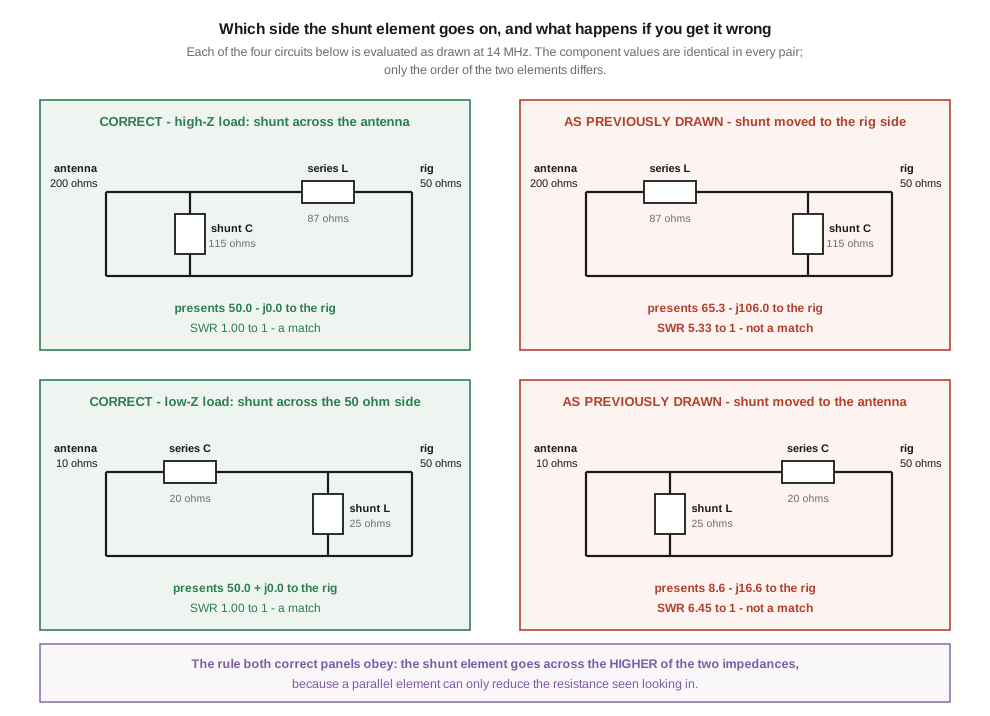
The correction that matters most is build-blocking. The previous edition printed the L-network design equations correctly and then drew both schematics with the shunt element on the wrong side of the series element. The equations give exactly 50 Ω; the drawings give 5.33:1 and 6.45:1. A reader who trusted the algebra was fine and a reader who followed the picture built a mismatch — and builders follow pictures. §2 derives which side the shunt belongs on from a single physical fact, so the rule is memorable rather than arbitrary.

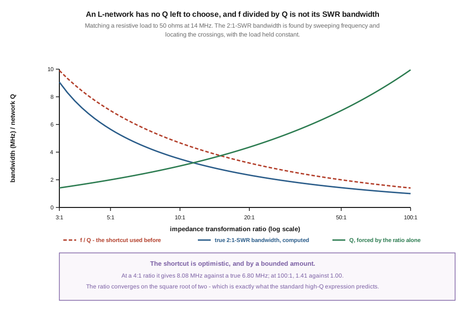
The second correction is smaller than it first looks, and saying so matters. The previous edition computed a “2:1-SWR bandwidth” as f/Q. That is the half-power bandwidth of a resonator, which is a different quantity — but §3 computes the true figure and finds the shortcut overstates it by only 19 % in the case quoted, converging to a factor of exactly √2 at high Q. The reasoning is wrong and the number is roughly right. Both halves of that sentence belong in the record.

The finding is about harmonics. A T-network is a high-pass filter and a pi-network is a low-pass filter, and that is not a curiosity — it is the reason vacuum-tube finals use pi-networks. §5 computes it: matched into the same load, the pi attenuates the second harmonic by 24.6 dB and the T by 1.2 dB. The most popular tuner topology in amateur radio provides essentially no harmonic protection, and none of the marketing mentions it.

2.2 The L-network, and which side the shunt goes on

An L-network is one series element and one shunt element. That is the whole thing, and it is the smallest network that can match an arbitrary resistive load to 50 Ω.

To see why the arrangement matters, notice what each element can and cannot do.

A series reactance cannot change resistance. Add jX in series with R + jX_load and you get R + j(X_load + X). The real part is untouched. A series element moves the reactance and nothing else.

A shunt reactance can only lower it. Put a reactance jX across a resistance R and the parallel combination has real part R·X²/(R² + X²), which is less than R for every finite X. A shunt element across a resistive load always reduces the resistance seen looking in, and can reduce it to any value you like by choosing X.

That single asymmetry determines the whole topology. The shunt element is the only one that transforms resistance, so it has to be placed where the resistance needs transforming — across the higher of the two impedances, bringing it down to the lower. The series element then cancels whatever reactance the shunt left behind. There is nothing else the two parts can do, and no other arrangement performs the job.

So the two orientations are:

• Load resistance above 50 Ω. The shunt goes across the load, pulling it down to 50 Ω. The series element sits between that node and the rig.
• Load resistance below 50 Ω. The shunt goes across the rig — the 50 Ω side is now the higher of the two — pulling it down to the load’s resistance. The series element sits between the load and that node.

Both cases obey the identical rule, which is worth stating because it is easy to memorise the two pictures separately and get them mixed up: the shunt element always goes across the higher impedance.

2.2.1 The equations, and what the previous edition drew

For a resistive load R matched to R₀ = 50 Ω, with R > R₀:

Q = √(R/R₀ − 1) X_series = Q·R₀ X_shunt = R/Q

and for R < R₀:

Q = √(R₀/R − 1) X_series = Q·R X_shunt = R₀/Q

Those equations, as the previous edition printed them, are exactly right. Worked at 14 MHz for a 200 Ω load: Q = 1.732, X_series = 86.6 Ω, X_shunt = 115.5 Ω — a 985 nH series inductor and a 98.5 pF shunt capacitor. Evaluate that circuit with the shunt across the 200 Ω load and it presents 50.00 − j0.00 to the rig. For a 10 Ω load: Q = 2.000, X_series = 20.0 Ω, X_shunt = 25.0 Ω, and with the shunt across the 50 Ω side it also presents 50.00 − j0.00.

Now evaluate the circuits the previous edition drew, using those same correct component values, with the shunt on the other side of the series element. The lead figure shows all four panels:

Table 1 — Now evaluate the circuits the previous edition drew, using those same correct component values, with the shunt on the other side of the series element. The lead figure shows all four panels

circuit	presents to the rig	SWR
200 Ω load, shunt across the load — correct	50.00 − j0.00	1.00:1
200 Ω load, shunt moved to the rig side — as drawn	65.31 − j106.04	5.33:1
10 Ω load, shunt across the 50 Ω side — correct	50.00 + j0.00	1.00:1
10 Ω load, shunt moved to the antenna — as drawn	8.62 − j16.55	6.45:1

The failure is not subtle and it is not a rounding matter. Built as drawn, either circuit is worse than no tuner at all in the sense that it has consumed two components, an afternoon and a chassis to produce a mismatch.

⭐ The general lesson is worth more than the specific fix, because this is the second dive in this program to need it. The random-wire and end-fed dive found a DIY section that specified a winding producing a 9:1 transformer in a build labelled 49:1, with the surrounding arithmetic entirely correct. Same shape: the numbers are right, the picture contradicts them, and a builder follows the picture. The rule that catches it is mechanical — verify a schematic by computing the circuit it draws, not by checking the equations printed beside it. Every schematic in this dive has been through that check, which is why the lead figure quotes an evaluated impedance under each panel rather than a claim.

2.2.2 There are four L-networks, not two

One more thing the previous edition missed. Each orientation has two valid element assignments, because reactance can be supplied by either an inductor or a capacitor. The 10 Ω match above can be made with a series capacitor of 20 Ω and a shunt inductor of 25 Ω, or with a series inductor of 20 Ω and a shunt capacitor of 25 Ω. Both are exact: both present 50.00 Ω.

They are not interchangeable in practice. One arrangement is a low-pass network and the other a high-pass, which matters for the same reason §5 develops at length. And they place very different demands on component values: at 3.7 MHz a 20 Ω series capacitor is about 2150 pF, which is not a component you will find in a tuner, while a 20 Ω series inductor is 0.86 µH, which is trivial. That constraint, rather than any principle, is what usually picks the arrangement.

2.3 The Q you do not get to choose

The Q in those equations is not a design parameter. It falls out of the impedance ratio and nothing else:

Q = √(ratio − 1)

A 4:1 transformation forces Q = 1.73. A 100:1 transformation forces Q = 9.95. There is no setting, no component choice and no cleverness that changes it, because the two-element network has no freedom left after the two matching conditions are met. The L-network’s Q, and therefore its bandwidth and a large part of its loss, are consequences of the job you gave it.

This is the L-network’s defining property, and it cuts both ways. It means you cannot accidentally choose a terrible setting — a virtue §4 will make much of. It also means that if the forced Q is too high for your purposes, an L-network offers you no way out.

2.3.1 What f/Q actually is

The previous edition wrote, of the 200 Ω example: “The Q is 1.73 — moderate, with 2:1-SWR bandwidth of ~14 MHz / 1.73 = 8 MHz at this frequency.”

f/Q is the half-power (−3 dB) bandwidth of a resonator of quality factor Q. It is a real and useful quantity and it is not a 2:1-SWR bandwidth. Those are different definitions of “bandwidth” — one is where the power falls to half, the other is where the reflection coefficient reaches one third — and identifying them is a conflation rather than an approximation.

So how wrong is the number? Sweeping the actual network — the 985 nH and 98.5 pF computed above, load held at 200 Ω resistive — the SWR passes 2:1 at 10.18 MHz and 16.99 MHz, a true bandwidth of 6.80 MHz. The shortcut said 8.08 MHz. It overstates by 19 %.

That is a much smaller error than the framing suggests, and it would be an over-correction to call the number wrong. What is going on is visible in the figure: the shortcut’s optimism grows with ratio and then stops, converging on a factor of √2. The reason is that the standard high-Q expression for the bandwidth between SWR limits is

BW = f₀ · (S − 1) / (Q · √S)

which for S = 2 is 0.7071 · f₀ / Q — precisely f/Q divided by √2. At high Q the computed sweep agrees with that expression to three figures. At the low Q of the worked example the high-Q approximation itself under-predicts, and the truth lands between the two. The previous edition’s arithmetic came out close by a partial cancellation of two errors.

2.3.2 The caveat that matters more than the arithmetic

There is a second problem with that sentence, and it is the one to carry away. A “6.8 MHz 2:1-SWR bandwidth at 14 MHz” is the bandwidth of the network driving a fixed 200 Ω resistor. No antenna does that. A real load’s resistance and reactance both move with frequency, usually far faster than the network’s response does, and on a wire antenna they can move by an order of magnitude across that span.

So the figure is a statement about the matching network in isolation, and it must not be read as “this tuner setting covers 10 to 17 MHz.” It does not. It says the network itself is not the thing that will limit you — which is genuinely useful, because it means that when a tuner setting stops working a few tens of kilohertz away, the network’s Q is not the reason. The antenna moved. That is the correct diagnosis and it is the opposite of the one an operator draws from a bandwidth number attached to the tuner.

2.4 The T-network, and the degree of freedom nobody tells you about

Add a third element and the counting changes. A T-network — series C, shunt L, series C — has three values to set against the same two conditions. Many different settings produce a perfect match, and they are not equivalent.

W9CF puts it plainly in the paper this dive leans on throughout: “Since there are only two matching equations, many combinations will provide a match. The optimum combination is the one that minimizes power loss.”

The figure below makes that concrete. It takes a 10 Ω load at 3.7 MHz, sweeps the output capacitor across its whole range, and for each value solves for the other two elements so that the input is exactly 50 Ω. Every point on the chart is a perfect match.

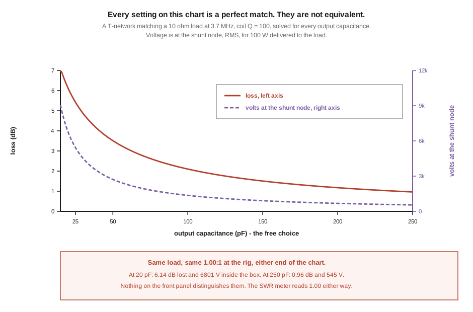
At 20 pF the network loses 6.14 dB — three quarters of the transmitter’s power — and stands 6 800 V RMS at its shunt node for 100 W into the load. At 250 pF the same network, matching the same load to the same 1.00:1, loses 0.96 dB and stands 545 V.

Both settings light the SWR meter at 1.00. Nothing on the front panel distinguishes them. And the second number is arguably the more alarming of the two: 6.8 kV inside a box whose air-variable capacitors are typically rated at a few kilovolts is not a loss problem, it is a flashover, and it happens at 100 W on a topology sold as handling a kilowatt.

2.4.1 The mechanism, stated correctly

The previous edition attributed the T-network’s loss to “the Q × resistance product dissipates more power per dB of forced match.” That is not a standard quantity and it does not name a mechanism. The real one is ordinary and is worth having, because it explains both the loss and the voltage at once.

W9CF’s analysis works in parallel equivalents, and the key observation is structural: “any T-network will transform the load resistance to a higher value which must also be higher than 50 ohms. It then transforms this high value down to 50 ohms to produce a match.” His worked example is a 10 Ω load at 80 m transformed to a 4 000 Ω parallel equivalent before being brought back down.

Now put the coil there. A real inductor’s loss appears as a parallel resistance of about Q·X_L, which for a good roller inductor at these frequencies is ten or twenty thousand ohms. Against 50 Ω that is negligible. Against the 4 000 Ω node the T-network has just created, it is not — and the fractional power lost is simply the ratio of the two. In his words, “the loss would be of order 10 percent, hardly negligible if a 1500 watt transmitter is used unless your coil is designed to dissipate 150 watts.”

That single picture explains everything on the chart. A smaller output capacitor means a higher intermediate impedance, which means more of the coil’s loss resistance in the path and more voltage across the node. Larger capacitors keep the intermediate impedance down. Hence W9CF’s operating rule, which is the single most useful sentence an operator of a manual T-network can know: the capacitors should be set to the largest value that still achieves a match.

The T-network model used to produce these figures reproduces all thirty-three cells of W9CF’s published loss table to within a few per cent, which is worth stating because two independent routes to the same numbers is better evidence than either alone. The full table, and what it does to the SWR-indexed loss figures the previous edition printed, is Vol 3’s subject.

2.4.2 The variants, and what they are for

Two common T derivatives exist specifically to manage this degree of freedom.

The differential T gangs the two capacitors so their values always sum to about the maximum, leaving the operator two controls instead of three. W9CF calculates it as a factor of two worse than a plain T at 1:1, converging to the same loss as the mismatch grows — and judges the trade worth it, because “one source of operator error is eliminated since a really bad set of component values cannot be chosen.” That is a design deliberately spending efficiency at the easy end to remove the failure mode the figure above illustrates.

The SPC transmatch connects a second section of the output capacitor across the coil. W9CF finds its loss is always greater than the standard T — 50 % more at 1:1, rising to double as the load resistance falls — and concludes there does not “appear to me to be any benefits from this circuit that offset this additional loss.” The ultimate transmatch adds a section across the input, where the reactance is large compared with 50 Ω, so it does almost nothing: the extra section “just increases the cost of the transmatch without improving it.”

2.5 The pi-network, and the filter you did not know you had

A pi-network is shunt C, series L, shunt C. It has the same three-elements-two-conditions structure as the T and therefore the same spare degree of freedom, and it is the standard output network of every vacuum-tube transmitter final ever built — the “tune” and “load” controls on a valve amplifier are the two capacitors of a pi.

That is not because a pi matches better. It is because of the shape of the circuit.

Look at the two topologies as filters rather than as matching networks. The T has series capacitors, which block low frequencies and pass high ones: it is a high-pass network. The pi has a series inductor with shunt capacitors to ground, which is the textbook low-pass. Both facts are visible on inspection, and both have consequences the amateur literature rarely draws out.

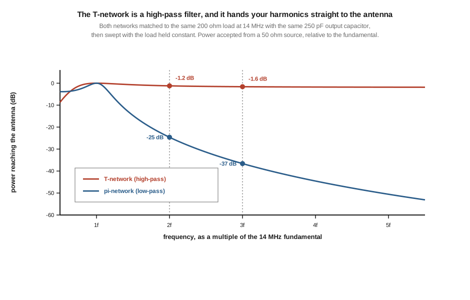
Matched to the same 200 Ω load at 14 MHz with the same 250 pF output capacitor, the two networks behave completely differently above the fundamental:

Table 2 — Matched to the same 200 Ω load at 14 MHz with the same 250 pF output capacitor, the two networks behave completely differently above the fundamental

	second harmonic	third harmonic
T-network	−1.2 dB	−1.6 dB
pi-network	−24.6 dB	−36.6 dB

The pi is a harmonic filter that happens to also match. The T passes harmonics essentially untouched.

Two caveats belong with those numbers. The load is held at 200 Ω resistive at every frequency, which no real antenna does; the exact decibels would move with a real load. And the conclusion does not depend on that, because it is a property of the topology rather than of the example — the T has a series capacitor between the transmitter and the antenna and cannot attenuate anything above its corner.

What follows practically is a matter of not giving credit where it is not due. A modern transceiver has its own low-pass filtering on each band and meets its spurious-emission requirements without help, so a T-network tuner passing harmonics is usually harmless. But it is not contributing, and the assumption that a tuner cleans up a signal is common and wrong. If you are running a homebrew transmitter, a tube amplifier without adequate output filtering, or anything whose harmonic performance you have not measured, the choice of tuner topology is a real decision and not a preference — and this is one of the few places in the hobby where the older technology is straightforwardly better at something.

2.6 Why the T dominates anyway

Given all that — a spare degree of freedom that can be set catastrophically, no harmonic attenuation, and a loss mechanism that gets ugly at low load resistances — the T-network is nonetheless the topology in almost every commercial amateur tuner. The reason is not marketing. It is match range with components that fit in a box.

Take the same parts and ask what each topology can actually match at 3.7 MHz, with capacitors of 250 pF maximum and a 30 µH coil:

• The T-network finds a match from a fraction of an ohm to about 19 kΩ.
• The L-network, in the configuration computed here, manages roughly 52 Ω to 9.6 kΩ.

The L-network’s failure is not a limitation of the topology — an ideal L-network matches anything. It is a component-value problem, and §2 already named it: matching a 10 Ω load at 3.7 MHz needs a series reactance of 20 Ω, which as a capacitor is about 2 150 pF. Air-spaced variables of that value with plate spacing for a kilowatt do not exist in any practical size. The T-network reaches those loads because its third element lets it get there with capacitors that do exist.

Add two more practical points and the market makes sense. Three independently switched elements are easy to automate — a relay bank on each is exactly how modern autotuners are built, and the topology’s tolerance of many solutions is a help to a search algorithm that only has to find one. And a manufacturer selling one box for 160 through 10 metres needs the widest reach it can get, because the customer’s antenna is unknown.

2.6.1 The correction to the correction

It would be easy to leave this section having concluded that the T-network is a lossy compromise. That is an over-correction, and W8JI is the necessary counterweight. His position is that “each network has advantages and disadvantages, while in actual fact loss differences are really fairly small”, and he offers the striking figure that “from 0 degrees to 130 degrees phase shift, a T-network with modest Q components has less than 0.1 dB loss!”

Both he and W9CF are right, and the apparent conflict is a difference of operating point. W9CF’s large numbers are for low resistances at 80 and 160 metres, where the intermediate impedance is highest and the coil’s finite Q bites hardest — his paper says so in its title. W8JI’s small numbers are for loads near 50 Ω, which is where most tuners spend most of their lives. A T-network trimming a resonant antenna’s band edges is doing almost nothing and losing almost nothing.

⭐ So the honest summary is not that the T is a lossy topology. It is that the T is a topology with a lossy setting, reachable at any time, indistinguishable from the good setting on every instrument the operator has. That is a different and more actionable statement, and it is why the differential T exists, why W9CF’s largest-capacitance rule is worth memorising, and why the loss question needs the whole of Vol 3 rather than a table.

2.7 Where this volume hands off

The counting argument carries the whole volume. Two conditions must be met to produce a match. A two-element L has exactly two values and therefore exactly one solution: no freedom, a Q forced by the impedance ratio alone, and no way to choose badly. A three-element T or pi has one value spare, which buys reach and automatability and costs the operator a choice they cannot see the consequences of. Within the L, the shunt element is the only one that transforms resistance, so it goes across the higher impedance — and the previous edition’s two schematics, which put it on the other side, produce 5.33:1 and 6.45:1 from equations that were exactly right. Between the T and the pi, the difference that matters most is not match range but the fact that one is a high-pass filter and the other a low-pass, worth 23 dB at the second harmonic.

From here:

• Vol 3 — Loss, and where to put the tuner takes §4’s degree of freedom and turns it into the dive’s central quantitative result. It replaces the previous edition’s SWR-indexed loss tables with W9CF’s measured and calculated work — which this volume’s model has already independently reproduced — and shows that the same 5:1 mismatch costs 1.00 dB into a 10 Ω load and 0.21 dB into 250 Ω. It then settles the shack-versus-mast-base question with the numbers Vol 1 §7 previewed.
• Vol 4 — Finding the load, and matching by hand turns §2’s algebra into geometry. The two moves of an L-network are two arcs on a Smith chart, the choice of orientation is a glance at which side of the chart your load sits on, and the whole of §2 becomes something you can do by eye once the picture is right.
• Vol 5 — DIY build and buys builds the 80–10 m L-network §2 derives, at 200 W, and surveys the commercial market — where the topology choices in this volume appear as product categories.

Nothing is owed against this volume: every figure is computed, every schematic has been evaluated as drawn, and the one external table it leans on has been independently reproduced.

2.8 Resources

• Kevin Schmidt, W9CF, Estimating T-network losses at 80 and 160 meters, QEX, July 1997 — the source for §4’s mechanism, the largest-capacitance operating rule, and the assessments of the differential T, the SPC and the ultimate transmatch. The paper’s host no longer resolves; it survives in the Internet Archive.
• Tom Rauch, W8JI, Antenna tuners — §6’s counterweight, and the source for realistic roller-inductor Q. Read alongside W9CF rather than instead of him; they are describing different operating points.
• ARRL, The ARRL Guide to Antenna Tuners — the book-length treatment of the topologies in this volume, and the standard reference for the network variants §4 surveys.
• David Pozar, Microwave Engineering, Ch. 5 — impedance matching and tuning from first principles, including the L-network’s two solutions and the Q-versus-bandwidth relationship §3 uses. The academic statement of everything in §2 and §3.
• Antenna tuners, Vol 1 — what the network is for, and why the SWR at the rig reports on the tuner rather than on the system.
• Random wire and end-fed antennas, Vol 5 — the other dive in this program whose DIY section drew a circuit its own arithmetic contradicted, and the reason §2’s verification rule exists.
• BALUNs and UNUNs, Vol 2 — the fixed-ratio transformer topologies, for comparison with the variable networks here.
• NanoVNA, Vol 4 — the S-parameter technique for measuring a network like these on the bench rather than trusting its front panel.