What a Tuner Actually Does

---

1.1 About this volume

An antenna tuner is the piece of equipment amateurs argue about most and understand least, and the two facts are related. It is a small box of inductors and capacitors performing an operation — impedance transformation — that has been fully understood since the 1920s and can be written down in two lines of algebra. Almost none of the argument is about the algebra. It is about what the box is doing to the rest of the system, and that question turns out to be genuinely subtle: subtle enough that two of the most careful writers in amateur radio spent three years disagreeing about it in the pages of QEX.

This dive covers variable-ratio matching networks — the tuner, the transmatch, the ATU, the antenna coupler, the matchbox. Its companion is the BALUNs and UNUNs dive, which covers fixed-ratio transformers: the 1:1, 4:1, 9:1 and 49:1 devices that match a specific antenna’s specific impedance. The dividing line is whether the impedance you are matching is known and stable. A resonant antenna at a design frequency presents a predictable impedance and a fixed transformer handles it. An antenna operated off resonance, or on a band it was never cut for, or fed with a length of open-wire line that transforms its impedance into something different on every band, presents an impedance that moves — and a fixed ratio cannot follow it.

This volume is about the thing itself: what the network does, what it reaches, and what it leaves untouched. The three canonical topologies and their design equations are Vol 2; loss, and the question of where in the system the tuner belongs, is Vol 3; measuring the actual load and matching it by hand is Vol 4; the build and the commercial survey are Vol 5.

Three of this volume’s conclusions run against what is usually said, and they are worth putting at the top rather than leaving the reader to find them.

The first is that a tuner reaches exactly one impedance in your system, and it is the one at its own input. It cannot change the antenna’s feedpoint impedance, and it cannot change the standing-wave ratio on the feedline. §3 shows this on a worked system where every figure is computed rather than asserted, and the numbers are unambiguous: the tuner produces a 1.00:1 match at the rig while the feeder it is connected to runs at 34:1, and no setting of the tuner alters the second number by any amount at all.

The second is that the famous conjugate match is real, is not quite what its defenders think it is, and does not matter. In a lossless system a tuner adjusted for a 50 Ω input does establish a conjugate match at every point in the system including the antenna feedpoint — §4 reproduces that exactly. It is also destroyed by a tenth of a decibel of feeder loss, and §4 shows which half of it goes first. The operator’s correct response to the whole question is the one G3TXQ gives: adjust for 50 + j0 at the tuner input, and stop thinking about it.

The third is the one to carry into every later volume: as the antenna system gets worse, every quantity visible from the operating position gets better. §7 sweeps feeder loss on a fixed system and finds that a worse feeder hands the tuner a lower SWR, which the tuner matches at a higher efficiency, in a shorter tune cycle — while the fraction of the transmitter’s power that reaches the antenna falls from 100 % to 20 %. Every instrument in the shack reports improvement. This is the same mechanism the random-wire dive found in its transformers, operating one level up, on the whole system.

1.2 The name is wrong, and the wrongness is load-bearing

A tuner does not tune the antenna. It does not change the antenna’s length, its resonant frequency, its radiation pattern, its efficiency, or the impedance it presents at its feedpoint. It is a two-port impedance transformer inserted in the line, and its entire function is to convert whatever impedance appears at its output terminals into 50 Ω resistive at its input terminals, so that the transmitter is presented with the load it was designed to drive.

This is not pedantry about vocabulary. The name is the source of most of the practical mistakes made with these devices, because it invites a specific and wrong mental model — that the tuner reaches down the feedline and does something to the antenna. Operators holding that model are surprised when a tuned system radiates poorly, conclude that the tuner is faulty, and buy a better one. The tuner was working perfectly. It was never the component in the loss path.

The hobby has better names and has never quite adopted them. Transmatch — a transmission-line matching network — is the ARRL’s own coinage and says what the device does. ATU, antenna coupler and matchbox are all in wide use. But antenna tuner is what the boxes say on the front panel and what the catalogues list, so it is the term this dive uses, with the understanding established here.

It is worth noting what the ARRL actually claims for the device, because it is a more careful statement than the folklore version. Its position is that “with proper system design, an antenna tuner or transmatch can allow a non-resonant antenna to operate nearly as efficiently as one that is carefully cut to resonance.” Read that closely. The claim is conditional on system design; it is about a non-resonant antenna rather than a bad one; and the comparison is to a resonant antenna of the same kind, not to an abstract ideal. It is a claim about the feed system, not about the antenna. Nothing in it says a tuner improves an antenna.

The distinction between “resonant” and “efficient” deserves stating once, plainly, because the two words get used interchangeably in casual conversation and they are unrelated properties.

Resonance is a statement about reactance: an antenna is resonant at the frequency where the reactive part of its feedpoint impedance passes through zero. Efficiency is a statement about where the power goes: the ratio of power radiated to power accepted. A full-size half-wave dipole in the clear is both resonant and efficient. A short loaded whip on a car roof can be trimmed to perfect resonance and remain one or two per cent efficient — the portable and mobile monopole dive works that case out in detail. A 40 m doublet used on 80 m is wildly non-resonant and, fed with low-loss open-wire line, remains a highly efficient radiator. Resonance is a convenience for the matching problem. It is not a measure of antenna quality, and a tuner’s ability to remove the matching problem says nothing whatever about the second question.

1.3 Three points in a system, and which one the tuner reaches

The clearest way to see what a tuner controls is to put a probe at three places in a real system and read what each says. The example that follows is Steve Hunt G3TXQ’s, used here because he chose it well and because every number in it can be — and has been — independently recomputed.

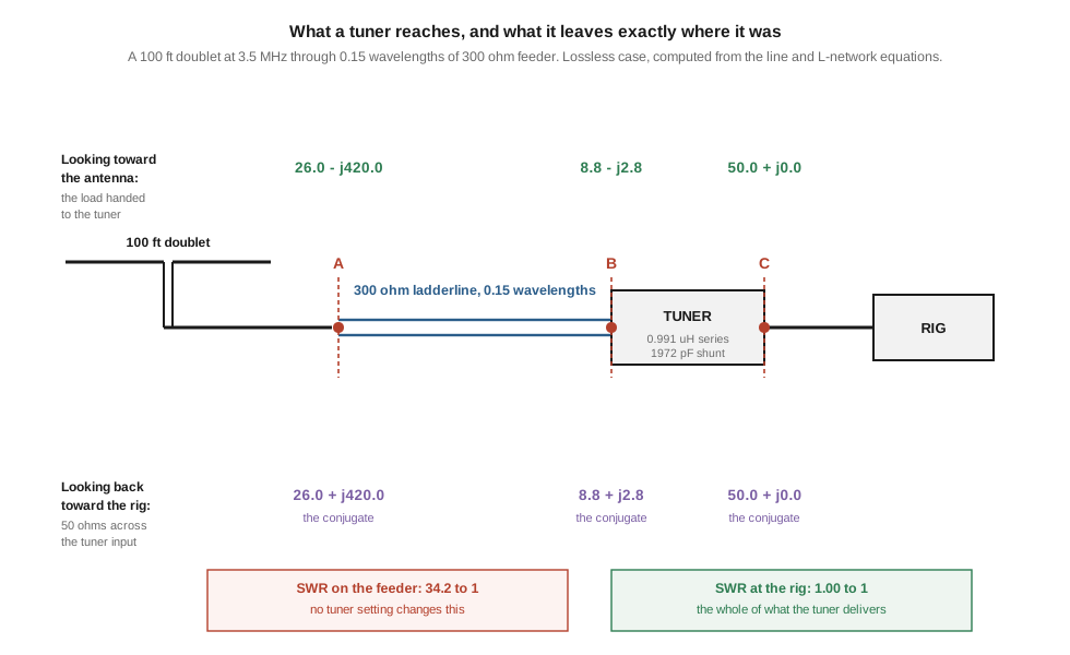
The system is a 100 ft doublet, centre-fed with 0.15 wavelengths of 300 Ω ladderline, working at 3.5 MHz into an L-network tuner. According to EZNEC the antenna’s feedpoint impedance is about 26 − j420 Ω: a strongly capacitive load a long way from anything a transmitter will accept. Label the antenna feedpoint A, the tuner’s output terminals B, and the tuner’s input terminals C.

Take the readings looking toward the antenna first. These are load impedances — what each stage is being asked to drive.

At A the analyser reads 26 − j420, the antenna’s own impedance. At B, after 0.15 wavelengths of 300 Ω line, it reads 8.77 − j2.78 Ω: the line has transformed the antenna’s impedance into something entirely different, which is what mismatched transmission lines do. At C, with the tuner set to 0.991 µH in series and 1972 pF in shunt, it reads 50.00 − j0.00 — a perfect match, exactly as designed.

Now repeat the exercise in the other direction. Replace the transmitter with a 50 Ω resistor, leave the tuner settings alone, and measure looking back toward the rig. These are source impedances — what each stage is being driven by.

At B the reading is 8.77 + j2.78. At A, after the same 0.15 wavelengths of line, 26.00 + j420.00.

Those are the conjugates of the forward readings, exactly, at every point. That is the result the lead figure shows, and it is the entire basis of the conjugate-match argument §4 takes up.

Two things about this system are worth holding onto before going further.

The feeder is running at 34.2:1. That is the standing-wave ratio a 26 − j420 load produces on a 300 Ω line, and the tuner cannot change it by any setting of any control. It is fixed by two things — the antenna’s impedance and the line’s characteristic impedance — and the tuner is party to neither. Meanwhile the rig sees 1.00:1. Both numbers describe the same system at the same instant, and an operator reading only the second has no information about the first.

One physical point carries two different SWR numbers. At the tuner’s output terminals the impedance is 8.77 − j2.78. Referenced to the 300 Ω feeder it sits on, that is the 34.2:1 already quoted. Referenced to 50 Ω — which is what a conventional SWR meter clipped in there would report — it is 5.72:1. Neither number is wrong; they answer different questions. SWR is not a property of a point in a circuit. It is a property of a point relative to a stated characteristic impedance, and a 50 Ω instrument inserted anywhere other than a 50 Ω line is reporting a quantity with no physical meaning at that location.

The practical summary is short. Looking at the figure: the tuner can change the reading at C and nothing else. At A and B it cannot touch the load impedance at all — though, as the next section shows, it does have an effect on the source impedance there, and that is a more interesting fact than it first appears.

1.4 The conjugate match — real, disputed, and beside the point

The conjugate match is the idea that when a tuner is correctly adjusted, every point in the system sees a source impedance that is the complex conjugate of the load impedance looking the other way: R + jX in one direction, R − jX in the other. The maximum-power-transfer theorem says this is the condition for maximum power delivery, so the conclusion drawn from it is attractive — adjust the tuner for a match at the rig and the entire system, right out to the antenna feedpoint, falls into optimal power transfer.

§3’s numbers say that is exactly true, at least in that example. And there is a clean structural reason for it, worth stating because it removes most of the mystery.

A lossless matching network that presents 50 Ω at its input necessarily presents the conjugate of its load at its output. This is not a special property of tuners; it is the standard lossless-two-port result. If the network dissipates nothing, all the power entering it leaves through the load port, which is the maximum-power condition at that port, which requires a conjugate match there. The conjugate relationship at B is not an achievement of the tuner. It is arithmetic, and it holds for any lossless network you could substitute.

So the interesting question is not what happens at the tuner’s terminals. It is whether the relationship survives the trip down the feedline to the antenna. That is where it falls apart.

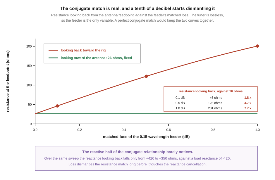
The figure sweeps one variable. The antenna is unchanged, the tuner is ideal and is re-adjusted for a 50 Ω input at every step, and only the feeder’s matched loss varies, from zero to one decibel. The quantity plotted is the resistance seen looking back from the antenna feedpoint, against the 26 Ω the antenna itself presents there.

At zero loss the two coincide exactly. At 0.1 dB — a feeder loss so small most operators would not bother to look it up — the source resistance is already 46 Ω against the load’s 26, a factor of 1.78. At 0.5 dB it is 123 Ω, a factor of 4.7. At 1 dB it is 201 Ω, a factor of 7.7. The system-wide conjugate match does not degrade gracefully. It is essentially gone by the time the feeder loses a quarter of a decibel.

What makes this more interesting than a general “losses spoil things” result is which half fails. Over that same sweep the reactance looking back moves only from +420 Ω to +350 Ω, against the load’s −420. The reactance cancellation is robust; the resistance match is fragile. The tuner goes on cancelling the antenna’s enormous capacitive reactance — the difficult and valuable part of the job — long after the resistive halves have stopped matching. That asymmetry is not usually mentioned in the argument, and it goes some way to explaining why systems keep working well past the point where the conjugate claim has stopped being true.

G3TXQ reached the same conclusion by a different route. Reworking his example with a real feeder (0.18 dB per 100 ft) and a real tuner inductor (Q of about 100), he found the impedance looking back at the antenna feedpoint became 45.7 + j421 against 26 − j420 looking forward, and wrote plainly:

Introducing realistic losses for the ladderline and the tuner has destroyed the “system-wide” conjugate match. There are some special cases where a “system-wide” conjugate match can occur even with a lossy system, but these are probably the exception in typical Amateur Radio installations.

His model is not identical to the one in the figure above — he evidently carries loss in a way that also moves the reactance at the tuner’s terminals, which the simpler model here does not — but the finding is the same, and the figure isolates the feeder as its sole cause.

1.4.1 The mechanism dispute, and why you can skip it

Running underneath all of this is a genuine technical disagreement about how a tuner establishes the match, worth knowing about mostly so that you can recognise it and decline to be drawn in.

Steve Best VE9SRB set out a wave-mechanics account in a three-part QEX series in 2001: that the rearward-travelling wave arriving at the tuner’s input port is “exactly equal in amplitude but 180 degrees out of phase with the source-voltage’s reflection at the T-network’s input”, so the two cancel and a 50 Ω steady-state input impedance results. Walter Maxwell W2DU disagreed in QEX for July/August 2004, arguing instead that two conjugately-related rearward waves interact to create a virtual open or short, re-reflecting all rearward power back toward the load. Jeff Anderson K6JCA later simulated an LC matching network and found the two voltages “equal in amplitude and opposite in phase” rather than conjugates, which supports Best’s account.

Note carefully what is and is not in dispute. Nobody involved doubts that the tuner produces a match, that the match is correctly predicted by the ordinary circuit equations, or that the equations in Vol 2 give the right component values. The argument is about which physical narrative correctly describes a steady state everyone agrees on. It has no bearing on how you set a tuner, what you buy, or where you install it — which is why this dive records it and moves on.

1.5 The transmitter is not a 50 Ω source

There is a second, independent reason the system-wide conjugate match is unlikely in practice, and it has nothing to do with loss. The conjugate argument requires the transmitter to behave as a Thévenin source whose internal impedance equals its specified load impedance: a 50 Ω generator behind a 50 Ω resistance. Modern solid-state HF transmitters are not that.

Warren Bruene W5OLY put the question directly in QST for November 1991, measuring the output source impedance of a tuned RF power amplifier by injecting a signal from a generator slightly off the operating frequency. He reported a source impedance of roughly five times the load impedance and concluded that a conjugate match did not exist. The measurement has been argued over ever since — the principal objection being that an off-frequency probe does not capture what the amplifier does to a reflected wave at its own operating frequency — so it belongs in the record as a contested result rather than a settled one. But the direction of the finding is not seriously disputed: a transmitter’s output impedance is not its rated load impedance, and there is no particular reason to expect it to be.

G3TXQ approached the same question from the operating end, running load-pull tests on two Ten-Tec Corsair IIs, an Omni VI and a pair of homebrew QRP transceivers. One of the Corsair IIs on 40 m produced “20% more power working into a load of 25+/-j21 (SWR(50)=2.4:1) than it did into a 50+j0 load.” That is a real and repeatable 0.8 dB, free, available to anyone willing to deliberately mistune the tuner.

His answer to whether one should take it is the right one, and it is the practical conclusion of this entire section:

Does that mean I should adjust the tuner to produce a conjugate match of 25-/+j21 at its input and thereby maximise the power from the radio? No - that would be ill-advised because the radio would not be operating into its specified load impedance, risking increased power dissipation and higher distortion products.

The extra power comes out of the amplifier’s headroom, and the price is paid in device dissipation and in intermodulation products landing on other people’s frequencies. The manufacturer specified 50 Ω because that is where the amplifier’s linearity, thermal and protection design all sit. Tune for 50 + j0 at the tuner input. That is the whole rule, and both reasons the conjugate match is unlikely — feeder loss and the transmitter’s actual source impedance — are reasons to stop worrying about it rather than reasons to chase it.

G3TXQ’s own summary of the tuner’s purpose is the plainest statement of it in the amateur literature: “The primary function of a tuner is to present the radio with its specified load impedance.” And on the conjugate question: “whether or not it also produces a ‘system-wide’ conjugate match - a most unlikely event - is of no concern!”

There is a corollary worth stating for anyone whose rig has a tuner built in. Manufacturers specify these by matching range, not by loss, and the ranges are narrow. Icom’s IC-7300 manual rates its internal tuner for mismatches up to 3:1, with a separate emergency mode that will attempt a match out to roughly 10:1 at a 50 W output ceiling. That is a design decision rather than a limitation of physics: a tuner living inside a transceiver has no room for large air-spaced components, so it is built to handle the common case and hand the rest to an external unit. Do not read a rig’s internal-tuner range as a statement about what tuners can do — and do not assume a published foldback threshold either, because the SWR at which a given radio starts reducing power is a per-model figure that has to be looked up rather than guessed at.

1.6 What a tuner cannot do

Most of this is implied by §3 now, but the list is worth making explicit because each item is a mistake that gets made.

A tuner does not change the antenna’s efficiency. If the antenna converts 3 % of the power it accepts into radiation, it does so with a tuner and without one. The tuner changes what the transmitter sees; it does not reach the radiating structure.

A tuner does not reduce the SWR on the feedline between itself and the antenna. §3’s system runs at 34.2:1 on the ladderline while the tuner produces a perfect match at the rig. This is the single most useful thing in this volume to internalise, because it is what makes the tuner’s placement a real engineering decision rather than a matter of convenience — which is Vol 3’s subject.

A tuner does not reduce feedline loss, and it usually cannot even see it. Worse, the high SWR it is silently accepting on the far side is amplifying that loss. In §3’s system a feeder with 0.10 dB of matched loss actually loses 1.44 dB at 34:1 — a factor of 14. The tuner reports none of this.

A tuner is not free. Its own components have finite Q and dissipate real power. How much is a more interesting question than the folklore suggests, and the usual way of presenting it — a table of “typical loss” indexed by SWR — turns out to be indexed against the wrong variable entirely. Vol 3 takes that apart with published measurements; the short version is that at a given SWR the loss can differ by more than a factor of ten depending on where on the constant-SWR circle the load actually sits.

A 1:1 reading at the rig is not evidence of anything except that the tuner is working. It says the transmitter is seeing 50 Ω. It says nothing about the antenna, the feeder, the efficiency, or the power actually radiated — and §7 shows that it can get better as all four of those get worse.

1.6.1 The one thing a tuner does do on receive

There is a genuine exception to “the tuner does not help”, and it is worth stating precisely because it is usually stated loosely. A tuner placed between antenna and receiver is a reactive two-port with a frequency response — it is, incidentally, a bandpass network. On receive it therefore acts as a modest preselector, attenuating signals well away from the frequency it is set for.

What that buys is improved resistance to front-end overload and to intermodulation products generated inside the receiver by strong out-of-band signals: a nearby broadcast transmitter, or your own second station. On a crowded low band with a wideband front end, that can be the difference between a usable receiver and an unusable one.

What it does not generally buy is a better signal-to-noise ratio on the wanted signal. HF reception below roughly 20 MHz is normally limited by external atmospheric and man-made noise arriving through the antenna rather than by the receiver’s own noise floor, and a passive filter attenuates the wanted signal and the noise arriving with it equally. The previous edition of this chapter claimed the preselector effect improves “the receiver’s signal-to-noise”, which attaches the wrong mechanism to a real benefit. The benefit is dynamic range, not sensitivity.

1.7 Every number you can see improves as the system gets worse

The last section of this volume is the one that motivates the rest of the dive, and it is a result rather than an argument.

Take §3’s system again — same antenna, same 0.15 wavelengths of 300 Ω feeder, same frequency — and sweep only the feeder’s matched loss from zero to one decibel, re-adjusting the tuner for a 50 Ω input at each step. Track three things: the SWR the tuner is handed at its output terminals, the fraction of power entering the feeder that reaches the antenna, and the tuner’s own efficiency with a lossless capacitor and an inductor of Q = 100.

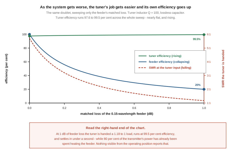
Table 1 — 7. Every number you can see improves as the system gets worse

feeder matched loss	SWR the tuner is handed	feeder efficiency	tuner efficiency
0.00 dB	5.72:1	100 %	97.6 %
0.10 dB	4.11:1	71.7 %	98.1 %
0.30 dB	2.63:1	45.8 %	98.6 %
0.50 dB	1.93:1	33.5 %	98.9 %
1.00 dB	1.18:1	20.0 %	99.5 %

Read the bottom row. With a decibel of feeder loss the tuner is handed a load that is already almost matched — 1.18:1, a figure most operators would be delighted with. It transforms that load at 99.5 % efficiency, the best number in the table. It will find the match in a fraction of a second and the tune cycle will feel effortless. And four fifths of the transmitter’s power has already been converted to heat in the feeder before the antenna sees any of it.

The mechanism is simple once stated. Loss attenuates the reflected wave as well as the forward one, so a lossy line presents at its input an impedance that has been dragged toward its own characteristic impedance — and, referenced to 50 Ω, toward a flattering SWR. The worse the feeder, the more thoroughly it hides the antenna behind it. In the limit, a sufficiently lossy line offers a beautiful match at every frequency and radiates nothing: it is the load.

This is precisely the finding the random-wire dive established for ferrite transformers — that loss flatters SWR, so the flattest sweep in a comparison may be the worst device in it — appearing one level up, at the scale of the whole antenna system. Same physics, same conclusion: an SWR reading taken on the transmitter side of a lossy element cannot certify anything on the far side of it.

Which is why the tuner is so persistently blamed for problems it did not cause and so rarely credited with the one thing it does. It is the most visible component in the chain and the only one with controls on it. It is also, on these numbers, running at between 97.6 and 99.5 % efficiency across the entire sweep — while the unglamorous length of wire feeding it throws away up to 80 %. The instrument panel in the shack reports on the tuner. Nothing on it reports on the feeder.

1.8 Where this volume hands off

The foundation is in place. A tuner is an impedance transformer, not an antenna adjustment. It reaches the impedance at its own input terminals and nothing else: the antenna’s feedpoint impedance and the standing-wave ratio on the feedline lie outside its reach entirely. It does establish a conjugate match at its own output, because any lossless network that matches in one direction does — but the system-wide version of that claim is destroyed by a tenth of a decibel of feeder loss, with the resistive half failing long before the reactive half, and it is undermined again by the transmitter not being a 50 Ω source. The operating rule survives all of it unchanged: adjust for 50 + j0 at the tuner input. And the numbers the operator can see are, by construction, the numbers least able to report on system health.

From here:

• Vol 2 — The three topologies derives the L, T and pi networks and draws them correctly. That word is doing real work: the previous edition of this chapter printed design equations that were exactly right beside two schematics wired backwards, and a builder following the drawings would have produced a 5.3:1 mismatch where the equations promised 1.00:1. Vol 2 also settles which side the shunt element belongs on and why, computes the real 2:1-SWR bandwidth of a matching network as against the resonator bandwidth f/Q the seed conflated with it, and explains why the T-network dominates the market despite costing more than an L in every respect except match range.
• Vol 3 — Loss, and where to put the tuner is where §7’s result gets quantified. It replaces the SWR-indexed loss tables with published measured work — which shows a 5:1 mismatch costing 1.00 dB into a 10 Ω load and 0.21 dB into 250 Ω, from the same network at the same SWR — and settles the shack-versus-mast-base question with numbers rather than rules of thumb.
• Vol 4 — Finding the load, and matching by hand turns the algebra into geometry: measuring what your antenna system actually presents, reading the two L-network elements off a Smith chart as two moves, and the cases where hand-matching still earns its keep against an autotuner costing less than a roller inductor.
• Vol 5 — DIY build and buys builds an 80–10 m L-network for 200 W and verifies it, then surveys what is worth buying. That survey has real work to do: the market the previous edition described no longer exists in the form it describes.

One item is owed against this volume and is recorded rather than skipped. The random-wire and end-fed dive links here for a per-band feedpoint impedance set on a multi-band end-fed — the 2450 Ω / 1500 Ω / 5000 Ω progression the seed chapter used as its opening example. Those numbers are a plausible illustration of the shape of the problem and are used in that spirit, but no source was found for them as measurements of any specific antenna, and the random-wire dive’s own §3 shows why any single quoted figure for an end-fed’s feedpoint is unreliable. A measured set from one real antenna across its bands would be a better example than an assumed one, and it is a bench task rather than a literature one.

1.9 Resources

• S. E. Hunt, G3TXQ, What tuners do — the worked doublet system §3 and §4 are built on, the load-pull measurements in §5, and the clearest statement of the tuner’s purpose in the amateur literature. Every lossless figure in it was independently recomputed for this volume and agrees exactly. His site’s certificate expired after his death in 2018; the page survives in the Internet Archive.
• Kevin Schmidt, W9CF, Estimating T-network losses at 80 and 160 meters, QEX, July 1997 — the calculated loss-versus-load work Vol 3 is built on, and the source of the observation that the constant-loss contours on a Smith chart are not the constant-SWR circles. Archived rather than live; the host it was published on no longer resolves.
• Steven Best, VE9SRB, Wave Mechanics of Transmission Lines, QEX, three parts, 2001 — the wave-mechanics account of how a tuner establishes a match.
• Walter Maxwell, W2DU, A Tutorial Dispelling Certain Misconceptions Concerning Wave Interference in Impedance Matching, QEX, July/August 2004 — the rebuttal, and the conjugate-match position in its strongest form. His book Reflections is the long version of the same argument.
• Jeff Anderson, K6JCA, Revisiting Maxwell’s Tutorial Concerning Wave Interference and Impedance Matching — a simulation of the disputed steady state, concluding for Best.
• Warren Bruene, W5OLY, RF Power Amplifiers and the Conjugate Match, QST, November 1991 — the source-impedance measurement discussed in §5. Cited here from secondary accounts rather than read first-hand; the original is worth obtaining before leaning on the specific factor of five.
• Tom Rauch, W8JI, Antenna tuners — the counterweight to W9CF on network choice, and the source for roller-inductor Q in real hardware.
• BALUNs and UNUNs, Vol 1 — the fixed-ratio half of the matching problem, and the natural companion to this dive.
• Random wire and end-fed antennas, Vol 4 — where loss flatters SWR was established for ferrite transformers, one level below §7’s system-scale version of the same effect.
• Antenna theory and practice — impedance, resonance, reflection coefficient and the Smith chart, if any of §3’s vocabulary needs shoring up.