Feed, Counterpoise and the Ground Question

---

4.1 About this volume

The three volumes before this one all end in the same place. Vol 1 derived a feedpoint resistance that is unbounded in the ideal case and said the real value must be measured. Vol 2 showed a fixed transformer ratio meeting a load that moves by nearly an order of magnitude across the bands, and deferred the loss question. Vol 3 audited wire lengths against a tuner’s reach and flagged a transformer target impedance it could not verify. Every one of them promised this volume.

So this is where the modelling stops. The subject is the feedpoint as an object you put an instrument on: what you actually measure there, how to pick a transformer ratio from that measurement rather than from a table, what the transformer costs you in decibels once you have picked it, and the two conductors — the counterpoise and the coaxial shield — that decide where the return current goes.

Four things structure it, and the first is the most important because it changes how you read every SWR figure in this dive.

Loss and mismatch are not distinguishable on an SWR meter, and loss makes mismatch look better. §5 computes the effect: a transformer with 2.3 dB of loss shows a 5:1 antenna as 2.29:1. That is not a subtle correction — it means the flattest sweep in a group of transformers may be the worst one in the group, and it means an SWR reading alone can never certify an end-fed system. A 50 Ω dummy load reads a perfect 1:1 and radiates nothing at all.

Core size buys cooling, not efficiency. The measurements in §4 span an eighteen-fold range of core mass and the loss moves by about a tenth of a decibel. Changing the material moves it by more than four decibels. The seed’s power table, which scales capability by core size, has the causation wrong: what a bigger core buys is surface area to shed heat, and that is a thermal argument rather than an efficiency one.

The counterpoise rule is not one rule. The seed’s own selection table says 5–10 % of the radiator for an end-fed half-wave and 50–100 % for a random wire, without explaining why the same component wants two wildly different lengths. §6 supplies the reason, because it is a real distinction rather than an inconsistency: those are two different jobs.

And a common-mode choke has to be resistive, not merely large. §7 computes what happens when a reactive choke lands on a reactive common-mode path: any inductive choke reactance from zero up to about +j400 Ω leaves more current on the braid than fitting no choke at all, on the path impedance this dive’s companion volume models. “Add a choke” is not automatically good advice.

4.2 The feedpoint you have, not the one you assumed

The previous edition’s selection table opens by describing a random wire’s feedpoint as 200–800 Ω (highly variable). Its own random-wire section, four pages earlier, describes the same quantity as ranging from 20 Ω to 5000 Ω. Both cannot be right, and Vol 3’s derivation says the second is closer: the feedpoint resistance of an end-fed wire follows 73/sin²(πm), which bottoms out at 73 Ω where the wire is an odd number of quarter-waves and runs away without limit near every half-wave multiple. A 200–800 Ω band describes a narrow slice of that range and would make the whole length-audit problem disappear.

For the resonant end-fed half-wave the same table says ~2450 Ω at resonance for all three cuts. Vol 1 established what that number is: 49 × 50, the ratio’s implication rather than a measured property, and a good system compromise rather than a constant. The measured picture, from the set recorded in the antenna tuners dive and the practitioner reports collected for this one:

Table 1 — For the resonant end-fed half-wave the same table says ~2450 Ω at resonance for all three cuts. [Vol 1](/random-wire-end-fed/vol-1/) established what that number is: 49 × 50, the ratio's implication rather than a measured property, and a good system compromise rather than a constant. The measured picture, from the set recorded in [the antenna tuners dive](/antenna-tuners/vol-1/) and the practitioner reports collected for this one

Where	Feedpoint resistance
One multi-band end-fed at 7 MHz	2450 Ω
The same antenna at 14 MHz	1500 Ω
The same antenna at 18 MHz	5000 Ω
An 80 m end-fed needing 20 secondary turns	nearer 5000 Ω than 2500 Ω
An 80 m end-fed on 10 m	as low as 600–1000 Ω

One antenna, a better-than-three-to-one spread, and the low figure is on the band a naive reading would predict to be highest. That last row is worth pausing on, because it inverts the intuition that a longer electrical length means a higher end impedance. It does not, reliably; loss, height, the transformer’s own stray capacitance and the wire’s surroundings all put their thumbs on the scale, and by the eighth harmonic they dominate.

The practical instruction is the boring one, and it is the reason this volume exists: put a vector instrument on it. A NanoVNA at the transformer’s antenna terminals, swept across the bands you care about, replaces every number in this section with numbers about your installation. The NanoVNA dive covers the calibration that makes such a measurement mean anything — and the calibration matters more here than in most places, because you are measuring kilohms with an instrument referenced to 50 Ω, which is the region where a sloppy calibration produces confident nonsense.

Two measurement cautions specific to this antenna:

• Measure at the transformer’s antenna side, not through it. Measuring at the coax end tells you what the system presents, which is what the transmitter cares about but not what you need in order to choose a ratio. The two questions want two different measurements.
• The instrument and its lead are part of the circuit at these impedances. Vol 1 recorded AF7NX’s finding that boxing a transformer and bringing its output through a connector raised the stray capacitance at that point to about 6.0 pF against roughly 1.6–2.7 pF for the bare winding. A few picofarads matters against a kilohm-scale source by the top of HF, and so does the way you attach the probe.

4.3 Choosing the ratio against a measured number

Once the feedpoint is a measurement rather than an assumption, ratio selection is arithmetic. A transformer of impedance ratio N² presents R/N² to the rig, and the SWR that results is R/(50N²) or its reciprocal. Vol 2 plotted the windows; the summary is that a 49:1 stays inside 2:1 for antenna resistances from about 1225 Ω to 4900 Ω, and a 64:1 for 1600 Ω to 6400 Ω.

Set the measured spread from §2 against those windows and the conclusion is immediate. No single fixed ratio covers a real multi-band end-fed’s whole range. An antenna running 1500 Ω on one band and 5000 Ω on another spans better than three to one; the windows are four to one wide; the two coincide only if the spread happens to sit almost exactly inside. The ratio is therefore a compromise chosen for the bands you care most about — not a correct answer waiting to be looked up, and not a component to keep swapping when one band misbehaves.

That reframes the seed’s selection table from a specification into a starting point, which is what it should have been. Rebuilt on that basis, and with the core column deliberately removed to Vol 5 where cores get proper treatment:

Table 2 — That reframes the seed's selection table from a specification into a starting point, which is what it should have been. Rebuilt on that basis, and with the core column deliberately removed to [Vol 5](/random-wire-end-fed/vol-5/) where cores get proper treatment

Antenna	Typical starting ratio	What to verify by measurement
Random wire, non-resonant	9:1	That the wire clears every half-wave multiple in your bands (Vol 3 §3), and that the tuner reaches what is left
End-fed half-wave, any cut	49:1	The per-band spread. If the bands you use cluster high, 64:1 is the better compromise
End-fed wire longer than λ/2	49:1 or 64:1	The actual feedpoint — see the flag below
Inverted-L, base-fed against radials	1:1, or direct	Feedpoint near 30–50 Ω, but dominated by ground-system quality rather than by the wire

⚠ The end-fed long wire row carries the flag Vol 3 raised and this volume cannot clear. The previous edition gives its feedpoint as “~3000–4500 Ω” and prescribes a 64:1. Note that 64 × 50 = 3200 and 81 × 50 = 4050, both inside the quoted bracket. This is the third target impedance in the dive to coincide with a transformer ratio times fifty, after the 2450 Ω and 3200 Ω cases that were traced to exactly that circularity and corrected. It is not being declared wrong — 4000 Ω is also quoted independently in amateur sources for full-wave end-feds, and declaring a real figure fictitious is a failure mode this program has committed before. What can be said is Vol 1’s conclusion: no formula produces it, the ideal model is unbounded there, and any specific number is a statement about a particular installation. Measure it.

4.3.1 The turns count is a separate decision from the ratio

A 2:14 winding, a 3:21 and a 5:35 are all 7:1 in turns and 49:1 in impedance, and they are not interchangeable. More primary turns means more magnetising inductance, which means the transformer intrudes less on what the transmitter sees; fewer turns means less winding capacitance and a better high-frequency limit. VK3IL states the rule that actually decides it: “as a rule of thumb you want at least 200 ohms on the transformer primary winding to avoid the transformer impacting the impedance seen by the transmitter too much” — which puts 3:21 or 3:24 on the low bands and 2:14 or 2:16 on the high ones. §4 is the evidence that this choice matters considerably more than the choice of core size.

4.4 What the transformer costs

Every volume so far has treated the transformer as an ideal ratio. It is not, and the size of the discrepancy is the most useful thing in this volume.

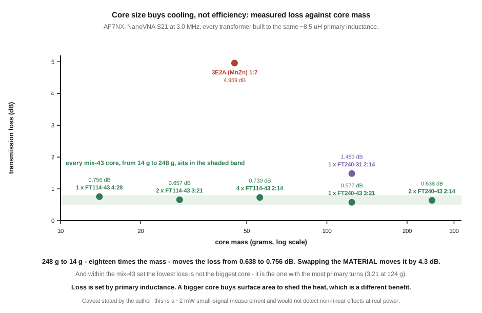
The lead figure plots AF7NX’s measured transmission loss for seven 49:1 transformers, all built to approximately the same 8.5 µH primary inductance, measured by NanoVNA S21 at 3.0 MHz with a documented de-embedding step for the 2400 Ω load. The result is not what a builder expects:

Table 3 — The lead figure plots AF7NX's measured transmission loss for seven 49:1 transformers, all built to approximately the same 8.5 µH primary inductance, measured by NanoVNA S21 at 3.0 MHz with a documented de-embedding step for the 2400 Ω load. The result is not what a builder expects

Core(s)	Turns	Core mass	Loss at 3 MHz
2 × FT240-43	2:14	248 g	0.638 dB
1 × FT240-43	3:21	124 g	0.577 dB
4 × FT114-43	2:14	56 g	0.730 dB
2 × FT114-43	3:21	28 g	0.657 dB
1 × FT114-43	4:28	14 g	0.756 dB
1 × FT240-31	2:14	124 g	1.483 dB
3E2A (MnZn)	1:7	45 g	4.959 dB

From 248 g down to 14 g — eighteen times the mass — the loss moves from 0.638 dB to 0.756 dB. In the author’s own words, “total heating power will be pretty much the same whether you are using a 250 gram core or a 14 gram core!” Meanwhile the lowest loss in the whole mix-43 set belongs not to the biggest core but to the one with the most primary turns for its size, and changing the material — the manganese-zinc core in the last row — costs 4.3 dB, thirty-six times the 0.118 dB that eighteen-fold change in size accounts for.

The mechanism is the one §3 already flagged: loss is set by primary inductance, and primary inductance is set by turns and material. A bigger core lets you reach a given inductance with fewer turns, and it gives you more surface area to get rid of the heat — but the heat produced is much the same. That dismantles the seed’s power table, which scales capability by core size as though a bigger core were more efficient. It is not more efficient; it is better cooled, which is a different and genuinely useful property, and it belongs in a thermal discussion rather than a loss one. Vol 5 takes it up there.

⚠ The author states a limitation and it should travel with the numbers. That measurement excites the transformer with about 2 mW, which puts the flux density far below any non-linear region, so “non-linear effects at real power would not have been detected.”

4.4.1 The check at real power

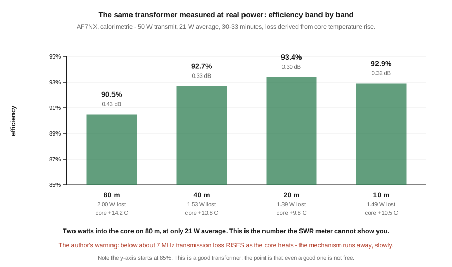
The same author’s calorimetric run closes that gap. An improved design — two FT114-43 cores, a five-turn primary, autotransformer-connected — driven at 50 W transmit, 21 W average, for 30 to 33 minutes, with loss derived from the core’s temperature rise:

Table 4 — The same author's calorimetric run closes that gap. An improved design — two FT114-43 cores, a five-turn primary, autotransformer-connected — driven at 50 W transmit, 21 W average, for 30 to 33 minutes, with loss derived from the core's temperature rise

Band	Temperature rise	Power into the core	Efficiency	Loss
80 m	14.2 °C	2.00 W	90.5 %	0.43 dB
40 m	10.8 °C	1.53 W	92.7 %	0.33 dB
20 m	9.8 °C	1.39 W	93.4 %	0.30 dB
10 m	10.5 °C	1.49 W	92.9 %	0.32 dB

This is the only real-power measurement in the set and it is the one to build on. Two watts of a twenty-one watt average is going into the ferrite on 80 m — 9.5 % of everything the transmitter produces, on a good transformer, at a power level most operators would consider modest. And the author’s accompanying warning is the one that matters for the low bands: “below about 7 MHz, transmission losses increase as the core temperature increases.” The mechanism has a slow positive feedback in it.

⚠ One source in this area is frequently misrepresented, including to me. PA3HHO’s widely cited page gives loss figures for single and double FT240-43 transformers — 2.3 dB on 80 m for a single core at 2:14, 0.8 dB for a double. Those are calculated, not measured: the page’s measurements are R, X and VSWR sweeps, and the loss numbers come from Owen Duffy’s ferrite-cored-inductor calculator. They also share that method with the other main published analysis, so the two agreeing is methodological consistency and not independent confirmation. The independent evidence is the two measurement sets above.

That said, the convergence does settle a contradiction the previous edition left open. Calculation and measurement agree that a single FT240-43 with a two-turn primary is a lossy transformer, which is exactly why the winding diagram this dive reproduces specifies “240-43, use min. of 2 cores” — while a table elsewhere in the same chapter rated one such core at 200 W SSB. The two-core minimum is about loss and heat; the single-core rating survives only on the low duty cycle of SSB speech.

4.5 Why a flat SWR curve can be bad news

Everything above has a consequence that is easy to state and easy to forget: a lossy transformer improves the SWR you measure.

An SWR meter at the shack end sees the reflection that comes back to it. A wave that goes out through a lossy transformer is attenuated on the way to the antenna, reflects, and is attenuated again on the way back. With a one-way power loss of L decibels the reflection coefficient seen at the input is

|Γ_in| = |Γ_ant| × 10^(−L/10)

— the exponent is L/10 rather than L/20 precisely because the wave makes the trip twice.

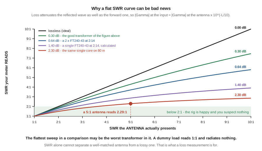
Worked through for the loss figures this volume has established:

Table 5 — Worked through for the loss figures this volume has established

One-way loss	A 3:1 antenna reads	A 5:1 antenna reads
0 dB (ideal)	3.00:1	5.00:1
0.30 dB (the good transformer of §4)	2.75:1	4.29:1
0.64 dB (2 × FT240-43 at 2:14)	2.52:1	3.71:1
1.40 dB (single FT240-43, calculated)	2.14:1	2.87:1
2.30 dB (the same single core on 80 m)	1.83:1	2.29:1

A 5:1 antenna behind a 2.3 dB transformer reads 2.29:1 — a figure most operators would accept without a second thought. The transmitter is happy, the tuner does not complain, and roughly forty per cent of the transmit power is being turned into heat in a ferrite core in a plastic box at the end of the garden.

Three practical consequences follow, and they are the reason this section exists rather than being a footnote:

• Never rank transformers by SWR flatness. In a comparison of several units into the same antenna, the flattest sweep is at least as likely to indicate the lossiest unit as the best-matched one. The limiting case is familiar: a 50 Ω dummy load is perfectly flat everywhere and radiates nothing.
• A “good SWR” is not evidence that an end-fed system is working. It is evidence that the transmitter is seeing something near 50 Ω, which a sufficiently lossy component guarantees regardless of what the antenna is doing.
• Loss has to be measured separately, by S21 through the transformer into a known load, or thermally, or by the substitution methods §4’s sources used. The NanoVNA dive covers the S21 technique; the specific fixture for a common-mode choke, which is a different measurement again, is in the BALUNs and UNUNs dive.

The honest version of the advice, then: use SWR to confirm the transmitter will run, and something else to confirm the antenna is radiating. They are separate questions, and only one of them has a meter on the front panel.

4.6 The counterpoise in practice

Vol 1 established what a counterpoise is for — it decides which conductor carries the return current, rather than adding gain — and gave the working figure of 5–10 % of the radiator’s length with the modelled support behind it. This section is the field version, and it starts with an apparent contradiction in the previous edition’s own selection table.

That table prescribes a counterpoise of 5–10 % of the wire for an end-fed half-wave, and 50–100 % of the wire for a random wire, with no explanation. It reads like an inconsistency. It is not: those are two different jobs, and the distinction is the most useful thing in the section.

• On an end-fed half-wave, the radiator is electrically complete. The wire is a full half-wave carrying its own standing wave, and the current at the feed is small — that is the whole reason the impedance there is high. The return path therefore handles a small current, and a short, deliberately non-resonant wire is enough to give it somewhere defined to go. Making it longer risks making it a resonant element, which drags the tuning around band by band and defeats the multi-band behaviour.
• On a random wire, the radiator is not complete, and the counterpoise is the other half of the antenna. Current entering the wire has to be balanced by real current in the return conductor, and that conductor radiates. A token wire will not do; the counterpoise needs to be a substantial fraction of the radiator, and it should be audited for half-wave collisions with the same arithmetic Vol 3 applies to the radiator.

Stated that way the two figures stop being contradictory and become a diagnostic: ask whether your radiator is a complete resonant structure. If it is, the counterpoise is a reference. If it is not, the counterpoise is half the antenna.

4.6.1 Length, and what actually tunes

For the end-fed half-wave case, AF7NX’s NEC study is the modelled support, and its four findings map directly onto practice:

• “‘Best’ results are with 2450 Ω drive impedance and the 3.3 m counterpoise” — on a 41 m wire that is 8 %, squarely inside the conventional 5–10 % band, and it is also the modelling result that makes the 49:1 convention a defensible system compromise rather than an accident.
• “With a very short counterpoise it is difficult to resonate the fundamental with any drive impedance” — the 3 % case is genuinely too short, so the lower bound is real rather than cautious.
• “Increasing the drive impedance tends to move the resonances to slightly higher frequencies” — the counterpoise and the transformer ratio interact, and should be chosen together rather than one after the other.
• Adding a further 2 m to the counterpoise moved the resonances very little — “much less than adding that length to the main wire would accomplish.”

That last one is the field rule and it is worth stating on its own: once the counterpoise is long enough to do its job, lengthening it is not a tuning control. Trim the radiator. A builder chasing a resonance by adjusting the counterpoise is adjusting the wrong wire, and the modelling says so explicitly.

For the common cuts that puts a 40 m end-fed’s counterpoise at roughly 1–2 m and an 80 m wire’s at 2–4 m.

4.6.2 The shield is already doing the job

The observation that stops a great many counterpoise experiments from making sense comes from VK3IL, answering a builder who found that adding a counterpoise changed nothing measurable: “with this type of matching unit, the coax shield essentially plays the role of a counterpoise, so adding a separate counterpoise is unlikely to make much difference.”

This is not an argument against counterpoises. It is the observation that you already have one, that it runs down the side of the house and into the shack, and that adding a second path does not automatically move current off the first. Which is why the next section is not a separate topic.

4.7 Common-mode current, the second device

A counterpoise offers the return current a path. It does not compel the current to take it. Making the unwanted path unattractive is a separate component’s job, and the two are one design decision.

The unwanted path is the outside of the coaxial braid. It is a conductor from the transformer, down the mast, along the ground and into the shack, and the current on it is what produces the two symptoms Vol 1 described: a raised receive noise floor, because that conductor is optimally routed for collecting house noise, and RF in the shack on transmit. A common-mode choke raises the impedance of that path.

The instinct is that more choking impedance is always better. It is not, and the reason is that the common-mode path has reactance of its own.

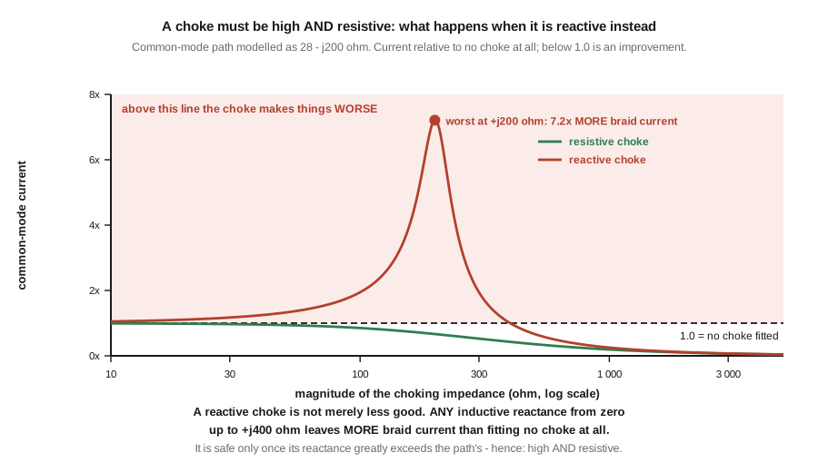
Take the common-mode path modelled in the BALUNs and UNUNs dive — 28 − j200 Ω, a magnitude of about 202 Ω, mostly capacitive reactance. The current on that path goes as the reciprocal of the total impedance, so:

Table 6 — Take the common-mode path modelled in [the BALUNs and UNUNs dive](/baluns-ununs/vol-1/) — 28 − j200 Ω, a magnitude of about 202 Ω, mostly capacitive reactance. The current on that path goes as the reciprocal of the total impedance, so

Choke fitted	Resulting path impedance	Common-mode current
none	202 Ω	1.00×
purely reactive, +j200 Ω	28 Ω	7.2× — much worse
purely reactive, +j500 Ω	301 Ω	0.67×
purely reactive, +j1000 Ω	800 Ω	0.25×
purely resistive, 200 Ω	303 Ω	0.67×
purely resistive, 1000 Ω	1047 Ω	0.19×

A purely inductive choke makes matters worse for every reactance from zero up to about +j400 Ω, because over that whole range it is partially or wholly cancelling the path’s capacitive reactance and lowering the total impedance. The worst case is exact cancellation, where the path collapses to its 28 Ω resistive part and the braid current rises more than sevenfold. Only once the choke’s reactance greatly exceeds the path’s does it start to help — and even then it helps less than the same magnitude of resistance would.

A resistive choke has no such failure mode. Adding resistance to 28 − j200 can only increase the magnitude, so the resistive curve falls monotonically from the first ohm.

Hence the rule, which is not “high impedance” but “high and resistive.” This is also, satisfyingly, the criterion that a ferrite’s complex permeability answers directly: the choking impedance is Z = ωμ₀N²(A_e/l_e)(μ″ + jμ′), so μ″ is the resistance and μ′ the reactance, and “resistive” reduces to μ″ > μ′ — a frequency-dependent property of the mix. That derivation, the mix data behind it and the measurement fixture that separates R from X belong to BALUNs and UNUNs Vol 3 and Vol 5 respectively, and are not duplicated here.

⚠ Two limits on the table above. It models the common-mode path as a single impedance and ignores the source, so it demonstrates the mechanism rather than predicting amperes — the modelled current figures for this specific case are in the companion dive. And 28 − j200 Ω is one modelled installation; the point is not that number but that the path has reactance, its sign and size are unknown to you, and a component whose benefit depends on their values is not a safe default.

The practical position for an end-fed system:

• Fit the choke at the transformer, where the boundary between antenna and feedline is, not at the shack end where the braid has already collected everything it is going to.
• Prefer a mix that is resistive at your bands over a mix with a bigger impedance number on a datasheet.
• Fit the counterpoise and the choke together. The choke makes the braid unattractive; the counterpoise gives the current somewhere better. Neither alone reliably does the job, and the failure to see any improvement from one is usually the absence of the other.
• Expect the improvement to show up as a quieter receive noise floor and a station that stops misbehaving at power — not as more signal report.

4.8 Where this volume hands off

The feedpoint is now something you measure rather than assume, and the consequences have been followed through. A real multi-band end-fed’s feedpoint resistance spans better than three to one across its bands and does not rise monotonically with harmonic number, so no fixed ratio is correct everywhere and the ratio is a compromise chosen for the bands you use. The transformer is not free: a good one costs 0.3 dB and puts two watts into its core at twenty-one watts average on 80 m, a mediocre one costs well over a decibel, and the difference is set by primary inductance rather than by core size — an eighteen-fold mass change moves the loss by about a tenth of a decibel while changing material moves it by more than four. That loss then hides itself, flattering the SWR reading until a 5:1 antenna reads 2.29:1. The counterpoise is short on a complete radiator and long on an incomplete one, because those are two different jobs, and the radiator rather than the counterpoise is what you trim. And a choke must be resistive as well as large, because a reactive one on a reactive path can multiply the current it was fitted to suppress.

From here:

• Vol 5 — DIY build, measurement and buys is the last volume and takes everything this one measured into the physical world: the build, the cut-and-trim procedure with a VNA, the core and winding choices this volume deliberately deferred, the power and duty-cycle question that §4’s thermal findings set up, and a dated commercial survey.
• Vol 1, Vol 2 and Vol 3 hold the derivations this volume put instruments on.

Four items are owed against this volume and are recorded rather than skipped. The end-fed long wire’s feedpoint impedance is still unverified — §3 flags the coincidence with 81 × 50 without declaring the figure wrong, and settling it needs a measurement nobody in the sourced literature appears to have published. No per-band feedpoint sweep of a specific antenna was available, so §2’s spread is assembled from several installations rather than measured on one. §7’s common-mode table is a mechanism model, not a prediction, and is labelled as such in place. And the figures here, like those in Vols 1–3, were verified numerically and by an XML bounds pass but never rasterised — the bounds pass caught a real overflow in this volume’s own caption during authoring, which is the argument for keeping it, but it is not a substitute for looking at them.

4.9 Resources

• AF7NX, Performance of 49:1 Ferrite Core Transformers (Squash Practice) — the NanoVNA S21 loss measurements plotted in §4, with the de-embedding step documented and the small-signal limitation stated by the author.
• AF7NX, Engineering the EFHW 49:1 Transformer and Antenna (Squash Practice) — the calorimetric efficiency measurements, the NEC counterpoise and drive-impedance study quoted in §6, and the stray-capacitance figures in §2. The most careful single treatment of this antenna’s feedpoint found for this dive.
• PA3HHO, Measurements and calculations on HWEF / EFHW transformers — the loss figures used as the high-loss end of §5’s table. ⚠ Calculated, not measured, and sharing a method with the other main published analysis, so not independent corroboration. Cited here for the shape of the result, not as evidence.
• VK3IL, EFHW matching unit — the 200 Ω primary rule in §3 and the coax-shield-as-counterpoise observation in §6. The comment thread is unusually good.
• BALUNs and UNUNs, Vol 1 — the common-mode path model §7 computes against, and the finding that a high but reactive choke can make things worse.
• BALUNs and UNUNs, Vol 3 — complex permeability, and the μ″ > μ′ criterion that §7’s “resistive” reduces to.
• BALUNs and UNUNs, Vol 5 — the series-through S21 fixture that measures choking impedance properly, which an SWR test into a dummy load cannot do at all.
• NanoVNA, Vol 3 and Vol 4 — calibration, and the S11 and S21 techniques §2 and §5 ask for.
• Antenna tuners, Vol 1 — the measured per-band feedpoint set in §2, and the tune-at-the-rig versus tune-at-the-antenna trade.