Calibration — the Discipline That Makes Every Later Reading Mean Something

---

3.1 About this volume

Vol 1 gave the reflection coefficient Γ and the S-parameter machinery their proper theoretical footing — what S11 and S21 mean for a 1-port and a 2-port DUT, how Γ maps onto the Smith chart, and why the whole apparatus is worth having. Vol 2 surveyed the hardware that implements it: the NanoVNA family’s generations, their dynamic range, their connectors, their firmware lineages. Neither volume asked the question this one exists to answer: how does a $50–300 instrument with a mediocre internal directional bridge, an imperfectly matched source, and a length of ordinary coax between its silicon and its test port ever produce a trustworthy complex number?

The answer is calibration, and it is worth being blunt about what that word is doing. Calibration on a VNA is not a courtesy step, not a “let the software settle” ritual, and not primarily about the antenna at all. It is a measurement of the instrument’s own imperfections, taken with standards whose electrical behavior is known (or assumed) precisely, so that the instrument’s imperfections can be subtracted — mathematically, exactly, term by term — from every measurement that follows. An uncalibrated NanoVNA does not measure your antenna badly; it measures the series combination of your antenna and the instrument’s own directivity error, source mismatch, and frequency response, with no way to tell you where one ends and the other begins. Calibration is the act of first measuring that combination against known references, solving for the instrument’s contribution, and then subtracting it out of every subsequent reading. Get it wrong, or skip a piece of the discipline, and every downstream number in this series — every SWR curve in Vol 4, every field trim decision in Vol 5, every S21 insertion-loss figure claimed for a BALUN or filter elsewhere in this hub — inherits the error without announcing it.

This volume owns the calibration discipline end to end: the error model that makes correction possible in the first place, the open/short/load (OSL) procedure that solves for it, what the through standard adds for a 2-port measurement, the reference-plane concept that decides where your corrected answer actually applies, the sweep-range and point-count constraints that bound a calibration’s validity, the quality question that separates a $20 stock kit from a lab-traceable one, the practical mechanics of saving and verifying a calibration, and the drift mechanisms that erode it in the field. It stops exactly where the corrected Γ is in hand and trustworthy. What you do with that trustworthy number — reading return loss and SWR off it, walking the Smith chart, running a TDR sweep — is Vol 4’s job. When and where in a deployment day to actually perform the calibration, and the field logistics of doing it at the top of a mast versus at the shack bench, belong to Vol 5. This volume is the theory that makes both of those downstream chapters honest.

3.2 The error model — what a 1-port measurement actually corrects

3.2.1 The naive picture is wrong

The naive mental model of a reflection measurement is disarmingly simple: send a known signal down the test port, measure what comes back, divide, and call the ratio Γ. If that were literally what happened inside the instrument, no calibration would ever be needed — the DUT’s true Γ would just fall out of the arithmetic. It isn’t what happens, and the reason is entirely mechanical. Between the NanoVNA’s synthesizer/receiver silicon and the SMA jack you actually connect things to sits a real, physically imperfect signal path: a directional bridge or coupler that is supposed to separate the outgoing wave from the returning one but never does so perfectly, a source whose output impedance is close to but not exactly 50 Ω, internal cabling and PCB traces with their own loss and phase response, and the connector itself. Every one of those imperfections contaminates the raw ratio the receiver reports, and every one of them is systematic — the same physical bridge, the same source, the same traces are there on every sweep, at every frequency, whether the DUT is a resonant dipole or a piece of open wire.

Systematic is the crucial word, because a systematic error, unlike random noise, can be characterized once and removed algebraically forever after — provided you have a model for exactly how it enters the measurement. That model is the whole content of this section.

3.2.2 The three-term error model

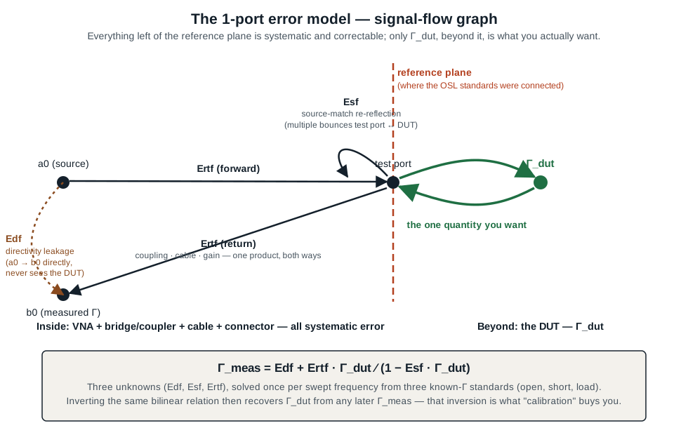
For a 1-port measurement, the standard result — developed identically for every VNA architecture from an HP 8753 to a NanoVNA, and derivable directly from a Mason’s-rule reduction of the instrument’s own signal-flow graph — is that the measured reflection coefficient Γ_meas relates to the DUT’s actual reflection coefficient Γ_dut by a single bilinear equation with three complex, frequency-dependent error terms:

Γ_meas = Edf + (Ertf · Γ_dut) / (1 − Esf · Γ_dut)

The three terms have clean physical readings, and each is worth sitting with:

• Edf — directivity. This is the fraction of the source signal that leaks straight into the reflection receiver without ever reaching the DUT — the directional bridge’s finite directivity, imperfect isolation between the forward and reverse coupling ports. Because it never sees the DUT, Edf is present even when Γ_dut = 0 exactly (a perfect 50 Ω load) — plug Γ_dut = 0 into the equation above and every term but Edf vanishes.
• Esf — source match. This is the reflection looking back into the instrument’s own source/bridge from the test port. Because the source is not a perfect 50 Ω termination, a wave that reflects off the DUT and heads back toward the source partially re-reflects, heads back out toward the DUT, reflects again, and so on — an infinite geometric series of internal bounces that the 1/(1 − Esf·Γ_dut) denominator sums in closed form.
• Ertf — reflection tracking (sometimes called frequency response). This is the net complex gain of the whole forward-and-return signal path — coupler coupling factor, internal cable loss and phase, receiver gain — that scales the DUT’s own Γ_dut up or down and rotates its phase, uniformly across whatever Γ_dut happens to be.

The figure below draws this as a signal-flow graph: directivity as a leakage path that bypasses the DUT entirely, reflection tracking as the forward-and-return gain that the DUT’s true Γ gets embedded in, and source match as a feedback loop representing the internal re-reflections. The reference plane — the physical point where the OSL standards get connected — is marked explicitly, because it is the boundary the entire correction is built around: everything to its left is instrument and cable, characterized once and subtracted; everything to its right is the DUT, and Γ_dut is the only thing beyond that line the measurement is actually trying to report.

3.2.3 Correction is inversion, not subtraction

Because the relationship between Γ_meas and Γ_dut is bilinear rather than additive, “removing” the error terms is not a matter of subtracting a fixed offset — it is solving the same equation for Γ_dut given a known Γ_meas and the three now-known error terms:

Γ_dut = (Γ_meas − Edf) / [Ertf + Esf · (Γ_meas − Edf)]

This is the single formula every subsequent S11 reading in Vol 4 is silently running through, once per swept frequency point, on every sweep, for as long as the calibration remains loaded. Everything from here forward is about how Edf, Esf, and Ertf get determined (§3), what changes when a second port and a through connection enter the picture (§4), why the answer those three terms produce is tied to a specific physical point in space (§5), why it is tied to a specific set of frequencies (§6), how good the standards used to solve for them need to be (§7), how you tell the resulting correction is trustworthy (§8), and how it erodes over time (§9).

3.3 The OSL procedure

3.3.1 Three standards, three unknowns

The three-term model has three unknowns per frequency point. Solving for three unknowns requires three independent equations, and the open/short/load (OSL) procedure supplies exactly that: connect a standard whose true Γ is known (or assumed) to the test port, record what the instrument measures, and repeat for two more standards whose known Γ is different enough from the first to make the resulting system of equations well-conditioned. The canonical choice — an open circuit, a short circuit, and a 50 Ω load — is not arbitrary; it places the three known points as far apart on the Γ-plane as physically realizable: Γ = +1 (open), Γ = −1 (short), and Γ = 0 (load), the two extremes of the unit circle and its center.

Substituting each standard’s known Γ into the bilinear model gives three equations in the three unknowns:

Γ_open,meas = Edf + Ertf/(1 − Esf) Γ_short,meas = Edf − Ertf/(1 + Esf) Γ_load,meas = Edf (exactly, when Γ_load = 0)

The load’s equation collapses immediately: if the load standard really does present Γ = 0, then whatever the instrument measures with the load connected is Edf, full stop — no algebra required. The open and short equations, now with Edf already known, are two equations in the two remaining unknowns Esf and Ertf, solved in closed form. This is worth stating plainly because it directly explains why §7 treats the load’s quality as the dominant variable: the load’s measured response is not one data point among three of equal weight — it is the direct, unmediated measurement of the directivity error term, and any real reflection the load itself contributes gets attributed entirely to Edf, corrupting the baseline every later measurement is referenced against.

3.3.2 What each standard is doing, physically

An open standard is, ideally, simply the absence of anything — an unterminated connector presenting a perfect total reflection with no phase shift beyond whatever the connector’s own mechanical length imposes. A short standard is a conductive plug bridging the center pin to the shield at (ideally) the same reference plane, presenting a perfect total reflection 180° out of phase with the open. A load standard is a resistive termination built to look, from the test port, exactly like an infinite length of 50 Ω transmission line — no reflection at all. Section 7 comes back to how far real hardware falls short of each of these ideals and why that gap is the entire quality axis of a cal kit.

3.3.3 Order, and what sloppy execution costs you

The instrument doesn’t care what order you connect the three standards in — the math is a simultaneous system, not a sequential one — but firmware UIs walk you through them one at a time (typically open, then short, then load) because each connection has to be individually confirmed and stored before the three equations can be solved together. What does matter enormously is the mechanical quality of each connection: a standard threaded on cross-threaded, torqued inconsistently, or contaminated with oxidation or moisture at the mating interface presents a Γ that differs from its nominal (or its published-definition) value in a way the calibration algorithm has no way to detect — it will solve the three equations exactly as written and produce error terms that are internally self-consistent but wrong, because they were solved against the wrong assumed inputs. A cross-threaded short, for instance, doesn’t fail loudly; it just shifts the effective reference plane by a fraction of a millimeter and adds a small residual reactance that the model attributes to Esf and Ertf rather than to the connector fault it actually is. The failure mode of a bad OSL connection is never an error message — it is a calibration that looks completely normal and is silently wrong, which is exactly why §8’s verification discipline exists as a mandatory step rather than an optional check.

3.4 What the through step adds

Everything in §§2–3 is the 1-port story, and it is the whole of what antenna S11 work needs. The moment the DUT becomes a 2-port device — a BALUN, a filter, a length of coax characterized end to end — the error model gains a second port’s worth of directivity, source match, and reflection tracking (six terms total, one triplet per port), plus terms that have no 1-port analog at all: a load match term for each direction (how well the far port, not just the near one, is terminated when it isn’t the one being driven) and a transmission tracking term (the net forward gain of the whole signal path from port 1’s source, through the DUT, to port 2’s receiver). The full accounting — twelve terms for a genuinely complete 2-port correction — also includes an isolation (leakage) term describing direct source-to-receiver coupling that bypasses the DUT on a 2-port instrument; most NanoVNA calibration routines assume this leakage is small enough to ignore and skip measuring it explicitly, which is a reasonable simplification for antenna and BALUN work but is exactly the kind of internal detail that belongs to Vol 2’s hardware treatment rather than being re-derived here.

The through standard — a short, known-good cable or direct mate connecting port 1 to port 2 — is what supplies the additional equations those extra terms need. Conceptually, it does for the transmission path what the load did for the reflection path in §3.1: it gives the instrument one measurement whose true value is known (a through connection is, ideally, S21 = 1∠0° and S11 = S22 = 0), letting the algorithm solve for the transmission tracking and load match terms the same way the OSL triplet solved for directivity, source match, and reflection tracking. Skip the through step, or perform it with a lossy or mismatched cable whose own insertion loss you haven’t accounted for, and every S21 measurement taken afterward silently includes that cable’s loss and mismatch as if it were the DUT’s own — a filter or BALUN will appear to have more insertion loss than it actually does, by exactly the amount the through standard itself was imperfect. The mechanics of actually reading and interpreting an S21 sweep once this correction is in place — insertion loss, group delay, the BALUN common-mode-rejection test — are Vol 4’s subject; this volume’s job ends at establishing that the through step is not optional bookkeeping but the second half of the same error-correction discipline the OSL triplet performs for reflection.

3.5 The reference plane in practice

3.5.1 Correction is exact — at one specific point in space

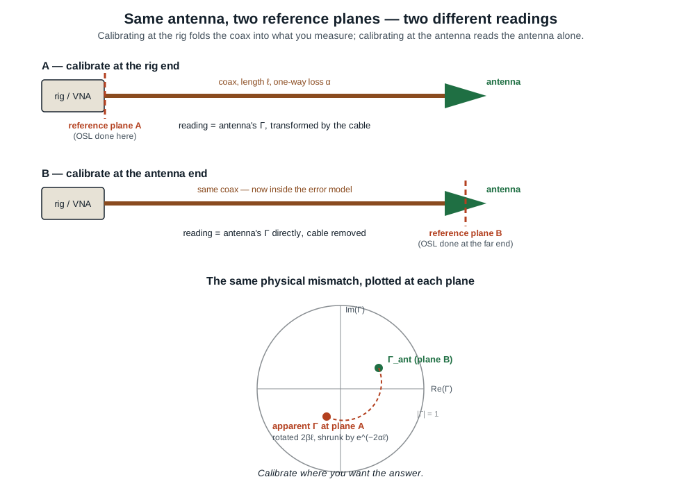
Every error term in §2’s model is defined relative to the physical point where the calibration standards were connected. Call that point the reference plane. The correction the instrument applies is not a general-purpose antenna-measuring algorithm; it is the specific algebraic undoing of whatever sits between the instrument’s internal receiver and that one physical connector face. Move the standards to a different point — the far end of a coax jumper instead of the NanoVNA’s own SMA jack — and you get a different, equally valid, equally exact correction, but one that answers a different question: what does the world look like from here rather than what does it look like from there.

This is worth stating as sharply as possible because it is the single most common source of a puzzled “why did my number change” moment: neither calibration configuration is wrong. A cal performed at the rig end of a coax run and a cal performed at the antenna end of the same run are both mathematically exact corrections of the instrument’s systematic error — they simply correct to two different reference planes, and a length of real transmission line sitting between those two planes transforms the reflection coefficient in a way that is itself entirely predictable, not an artifact of doing something incorrectly.

3.5.2 The transformation a length of line performs

A transmission line of physical length ℓ, propagation constant γ = α + jβ (α the attenuation per unit length in nepers, β the phase constant), terminated in a load of reflection coefficient Γ_L, presents at its input end a reflection coefficient

Γ_in = Γ_L · e^(−2γℓ) = Γ_L · e^(−2αℓ) · e^(−j2βℓ)

— the standard transmission-line result for how a reflection coefficient transforms along a lossy line (Pozar, Microwave Engineering, develops this directly from the line’s forward- and backward-traveling wave solution). Read the two exponential factors separately, because they do different things to the point on the Γ-plane. The phase term e^(−j2βℓ) rotates Γ_L by twice the line’s electrical length — the familiar fact that walking a matched reference plane down a lossless line traces a circle of constant |Γ| on the Smith chart. The magnitude term e^(−2αℓ) shrinks |Γ_L| toward the origin by twice the line’s one-way attenuation (in dB, the total round-trip loss). Together, calibrating at the rig end and then inserting a real coax run between the calibrated reference plane and the antenna does not just relabel the same number — it moves the plotted point along an inward spiral, rotated and pulled toward the chart’s center.

For illustration only — not a measured or vendor figure, just the arithmetic the formula above implies — suppose a coax run has a modest one-way matched-line loss of 0.5 dB (a plausible ballpark for a moderate length of good HF coax at the frequencies this hub’s dipole and vertical volumes discuss). The round-trip attenuation is 1.0 dB, and the magnitude scaling factor is 10^(−1.0/20) ≈ 0.89. An antenna presenting a genuine |Γ_ant| = 0.20 at its own feedpoint (roughly a 1.5:1 SWR) would appear, measured through that same cable with the calibration left at the rig end, as |Γ| ≈ 0.18 — a smaller, better-looking number, for no reason connected to the antenna’s actual match. This is precisely the same phenomenon Vol 1 of the fixed-vertical-monopoles dive flags from the opposite direction — a lossy ground system can make a mismatched vertical’s SWR look artificially flattering by burning the reflected power as heat rather than reflecting it — and it is worth internalizing as a general rule: any lossy element between the true reference plane and the point you actually calibrate at will make the reading look slightly better than reality, never worse.

3.5.3 Calibrate where you want the answer

That single sentence is the entire discipline. If the question is “what does my rig’s matching network see, coax and all” — the practical question for setting up an antenna tuner or checking a transceiver’s load tolerance — calibrate at the rig end; the coax’s contribution belongs in that answer. If the question is “is this antenna itself resonant and well matched” — the design and trim question this entire hub’s per-antenna volumes are built around — the coax’s loss and phase rotation are noise you do not want folded into the number, and the calibration standards belong at the antenna’s own feedpoint, using the identical coax (and any adapters) that will carry the signal in the final measurement. There is no universally “more correct” choice between the two; there is only a mismatch between which reference plane you calibrated at and which one the question you’re actually asking requires.

3.6 Sweep range, point count, and the cal’s validity

3.6.1 A calibration is a table, not a function

Section 2’s error model is continuous in frequency in principle, but the instrument never solves it continuously — it solves the three-equation (or twelve-equation) system independently at each discrete frequency in the swept grid, and stores the result as a table: one row per swept point, each row holding that point’s own Edf, Esf, Ertf (and, for a 2-port cal, the rest of the twelve). The frequency grid itself is entirely determined by three numbers — start frequency, stop frequency, and point count — because those three fix every discrete frequency the sweep actually visits. The calibration is valid only at the exact rows in that table; it says nothing, by construction, about any frequency that was never swept during the OSL/through sequence.

3.6.2 What changing the span does

Change the start frequency, the stop frequency, or the point count after calibrating, and the new sweep’s frequency grid is, in general, a completely different set of points from the one the calibration table was built against. A point that happens to coincide exactly with an old calibrated row is still correctable; every other point falls between rows that were characterized, or outside the range that was characterized at all. Firmware handles the two cases differently, and it is worth being precise about which is which rather than treating “changing the span” as one undifferentiated hazard. For a new frequency that falls within the original calibrated span but off its exact grid, most NanoVNA firmware families interpolate the stored error terms from the two bracketing calibrated points — a reasonable approximation where Edf, Esf, and Ertf vary smoothly with frequency (true across most of an HF sweep), and a worse one anywhere those terms change quickly (near a cable or connector’s own resonances, or toward the edges of the instrument’s usable range). For a new frequency that falls outside the calibrated span entirely, there is no bracketing data to interpolate from at all, and the safer firmware behavior — which is what most current NanoVNA lineages do — is to flag the calibration as invalid for that sweep and revert to raw, uncorrected data rather than extrapolate silently past error terms that were never actually measured out there.

Either way, the practical rule is the same: treat a change to start, stop, or point count as a mandatory re-calibration, not an optional one. This is distinct from a change to IF bandwidth or averaging, which affects how noisy the measurement itself is at each point but does not move the frequency grid the calibration table is indexed by — a change worth keeping conceptually separate rather than lumping together as “anything you touch invalidates the cal,” which overstates the mechanism and obscures the actual reason (grid mismatch, not settings in general).

3.7 Calibration-kit quality

3.7.1 What a stock kit’s three pieces actually are

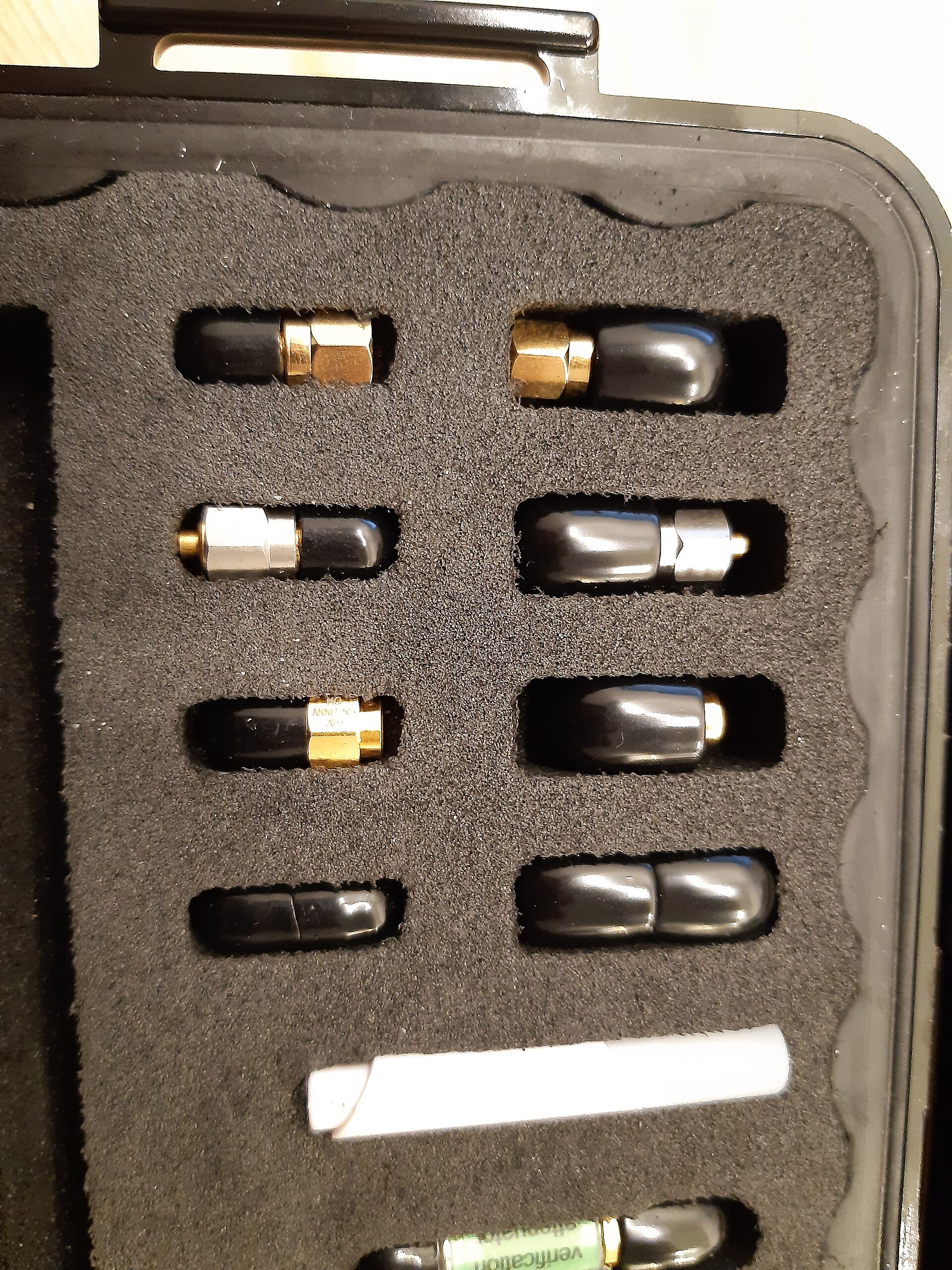
The calibration kit that ships with a typical budget-to-mid-tier NanoVNA is unglamorous, and it is worth being concrete about what is actually inside the three (or six, for a 2-port set with both connector genders) small metal pieces. The open is, physically, just an unterminated SMA connector — no cap, no component, simply the bare jack presenting whatever fringing field forms at its open end. The short is a small conductive plug that bridges the center pin to the shield as close to the connector’s mating plane as the mechanical design allows. The load is a thin-film or SMD chip resistor, soldered across the center conductor and ground inside a small SMA housing, whose only claim to “50 Ω” is the resistor’s own manufacturing tolerance plus whatever parasitic inductance and capacitance the mounting geometry adds. None of this is a criticism of the concept — it is the correct physical realization of all three standards — the quality question is entirely about how precisely each piece matches its ideal, and how well that deviation is characterized.

3.7.2 Offset delay and why the ideal ±1 assumption breaks down

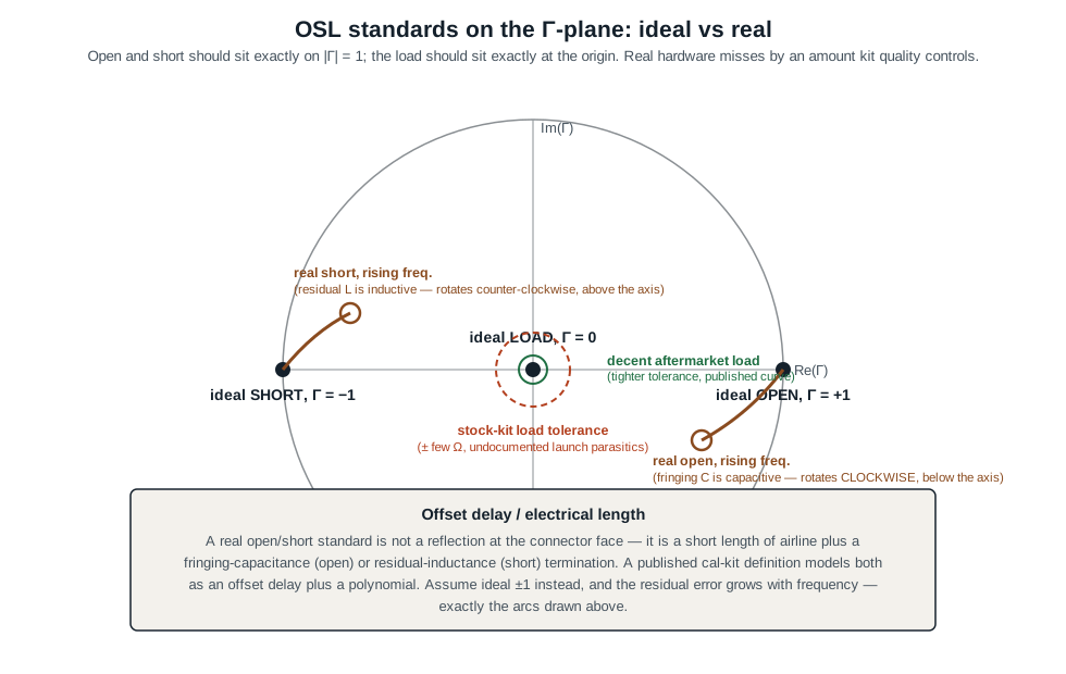
A real open standard is not a perfect Γ = +1 at every frequency: the connector’s mechanical length between the reference plane and the point where the field actually terminates behaves as a short section of transmission line (an “offset delay,” typically specified in picoseconds), and the open end’s fringing capacitance adds a small frequency-dependent phase shift on top of that — the open drifts off the +1 point as frequency rises, tracing a small arc around the unit circle rather than sitting fixed on the real axis. It is worth separating two effects that the figure below shows together, because only one of them is what most treatments name. Offset delay and fringing capacitance are both lossless — a purely reactive termination has |Γ| = 1 exactly, and a lossless line segment rotates Γ without changing its magnitude — so neither can move a standard inside the unit circle. What does is offset loss, the resistive and dielectric loss of the standard’s own short airline, which lab-grade kit definitions specify as a separate parameter alongside the delay. The rotation is the delay and the fringing C; the inward shrink is the loss. And the directions are opposite for the two standards: the open’s fringing capacitance is capacitive, so it rotates clockwise below the real axis, while the short’s residual series inductance rotates it counter-clockwise above. The short has the mirror problem: the physical short-circuit plane sits a small offset delay away from the true reference plane, and the connector geometry adds a small residual series inductance that likewise rotates the ideal −1 point off the real axis as frequency climbs. Professional cal-kit definitions (the parameter sets Keysight, Agilent, and other lab-grade vendors publish for their own kits, entered into the calibration software as an offset delay, an offset loss, an offset impedance, and — for the open specifically — a fringing-capacitance polynomial) let the calibration algorithm solve the three-equation system against each standard’s true, frequency-dependent Γ rather than an assumed ideal ±1. A calibration that instead assumes ideal standards throughout — which is what happens by default with an unspecified or undocumented kit — accumulates exactly the residual error those offset terms exist to correct, and because the physical effects (fringing capacitance, connector electrical length) both grow with frequency, the resulting error is smallest at the low end of a sweep and worst at the top — the practical reason cheap-kit accuracy is reported to degrade well before an instrument’s own frequency ceiling, though the specific frequency at which that degradation becomes noticeable depends on the particular kit and cannot be stated as a fixed number without a kit-specific definition file in hand.

3.7.3 Why the load matters most

Section 3.1 already derived the reason algebraically: the load standard’s measured response, if the load is truly Γ = 0, is the directivity error term with no further computation required. Any real reflection the load itself contributes — from resistor tolerance, from the parasitic inductance/capacitance of its mounting geometry, from a launch discontinuity where the connector meets the resistive element — gets attributed entirely to Edf rather than flagged as “load imperfection,” and Edf is the term that sets the floor every subsequent measurement is referenced against. A dead-flat 50 Ω load whose true Γ grows with frequency (a common failure mode for a cheap chip-resistor termination, whose parasitic reactance becomes a larger fraction of 50 Ω as frequency rises even when the DC resistance is dead-on) corrupts precisely the low-Γ region of the measurement — which is exactly the region a well-matched, well-trimmed antenna’s own S11 lives in. An imperfect open or short mostly costs you accuracy at the edges of the Smith chart, where high-SWR conditions live; an imperfect load costs you accuracy at the center, where a good antenna’s reading is supposed to land.

3.7.4 Stock kit, aftermarket kit, and the honest price ladder

At the entry end, the stock kit bundled with a budget NanoVNA — the Nooelec NanoVNA-H4, for instance, ships with what its own product listing describes only as a “3pc SMA calibration kit” / “SOLT SMA calibration kit,” with no offset delay, tolerance, or frequency-response specification published for any of the three pieces. That opacity is itself the point: a stock kit’s manufacturer is not publishing a definition file because the components are not individually characterized to a level worth publishing — you are trusting nominal geometry and connector tolerance, nothing more.

At the far end of the market, professional mechanical calibration kits from a metrology-grade vendor are individually characterized, come with certificates, and are priced accordingly. Copper Mountain Technologies’ current SMA-family mechanical calibration kits (verified live against their own calibration-kits product page) run from $595 for a DC–1.5 GHz kit up to $1,845–$2,305 for kits rated to 18–26 GHz — pricing that reflects individually measured, traceable standards rather than nominal parts, and that is aimed squarely at instrument houses and metrology labs rather than the amateur antenna bench.

Between those two extremes sits a real but harder-to-pin-down middle tier: SMA OSL kits marketed specifically at hobbyist VNA and NanoVNA users, typically in the tens of dollars, promising tighter mechanical tolerance and sometimes a published nominal offset-delay figure without the full metrology-grade characterization certificate a Copper Mountain kit carries. This review could not confirm a specific current product or price for that tier live — treat it as a real category rather than an endorsement of any particular listing, and verify any specific SKU’s price and spec sheet before buying. It is also worth flagging that earlier drafts of this dive’s source material cited specific Mini-Circuits and Picotest cal-kit part numbers and prices; a live check of Mini-Circuits’ own product catalog turned up no dedicated calibration-kit product line at all (their business is RF components — amplifiers, mixers, splitters — not calibration standards), so those specific claims could not be verified and are not repeated here.

3.7.5 The honest diminishing-returns case

For the antenna work this hub is built around — HF S11 sweeps looking for a resonance dip and a reasonable SWR bandwidth, using the trim-and-sweep workflow Vol 5 develops — the stock kit’s few-percent load tolerance and low-picosecond offset errors are almost always smaller than the other error sources already in the measurement chain: ground proximity effects on the antenna itself, cable flex between sweeps, the SMA connector’s own several-hundred-cycle wear budget (§9.2), and ordinary temperature swings across a field session. An aftermarket or lab-grade kit earns its keep in a narrower set of cases: characterizing a filter or BALUN’s insertion loss to a few hundredths of a dB, working meaningfully into VHF/UHF/microwave territory where the stock kit’s uncharacterized parasitics have had more frequency to accumulate phase error, or producing results that need to stand up to an external, traceable standard rather than an internal, self-consistent one. Chasing calibration-kit precision on a single-band HF dipole or vertical is effort spent for a return that is already buried under bigger, uncorrectable sources of variation elsewhere in the measurement. Spend the marginal dollar on a better antenna or a cleaner ground system before spending it on a better cal kit.

3.8 Saving, recalling, and verifying a calibration

3.8.1 What save and recall actually preserve

Saving a calibration preserves exactly the table §6.1 describes: the frequency grid the OSL (and, for 2-port work, through) sequence was executed against, and the resulting error-term coefficients at each of those frequencies. Recalling a saved calibration restores that table and applies it to whatever sweep the instrument is currently running — provided, per §6.2, that the current sweep’s frequency grid actually matches (or falls inside, for the interpolated case) the grid the saved table was built against. What save/recall does not do is validate that the underlying calibration was any good in the first place: a calibration performed with a cross-threaded short, a marginal load, or a cal kit whose standards were never actually removed and reconnected between steps saves and recalls exactly as cleanly as a good one. The mechanics of which memory slot holds what, and how many slots a given NanoVNA model provides, are hardware-UI details that belong to Vol 2; the discipline point that belongs here is that a saved calibration is only as trustworthy as the connections that produced it, and neither the save operation nor the recall operation can tell you which kind you have.

3.8.2 The verification trap: don’t check the cal against itself

The single most important — and most commonly skipped — step in the entire calibration discipline is verifying the result against an independent standard, one that was not part of the OSL (or through) set just used. The reason is structural, not a matter of carefulness: because the three-term model was solved as an exact system of three equations in three unknowns using the open, short, and load measurements themselves, re-measuring any one of those same three standards after calibrating is mathematically guaranteed to reproduce its assumed ideal value exactly, regardless of how badly the calibration actually went. Reconnect the load standard you just calibrated with and read a perfect Γ ≈ 0 — that is the algebra working as designed, not evidence the calibration is good. Verifying a calibration by re-measuring one of its own three standards proves nothing.

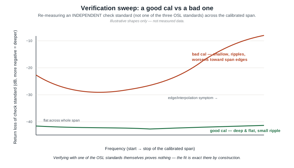
A meaningful verification needs a standard whose true response is known but which was held back from the calibration itself — a second, nominally-identical load if you own two, a different physical open or short than the one just used, or (closer to what a metrology lab would use) a precision fixed attenuator terminated in a good load, whose small, calculable, non-zero reflection gives you something to check both magnitude and phase tracking against across the swept band, rather than a trivial null. What a good calibration’s verification sweep looks like is a deep, comparatively flat trace with only modest ripple across the calibrated span, sitting well below the level any real antenna or filter measurement will be reading; what a bad calibration’s verification sweep looks like is shallower than expected, and — consistent with §6.2’s interpolation mechanism — often worse specifically toward the edges of the calibrated span rather than uniformly across it. Both patterns are illustrated schematically below; the specific dB numbers are representative only, not a measured result, since the actual depth achievable depends on the instrument’s own dynamic range as much as on the calibration quality.

3.9 Calibration drift

A calibration is a snapshot: it characterizes the instrument’s error terms as they existed at the moment the OSL (and through) standards were connected. Nothing about the underlying hardware promises to stay in that exact state, and three mechanisms in particular erode a calibration’s accuracy over the course of a real measurement session.

Thermal drift comes from the same physics that makes any RF hardware temperature-sensitive: the coupler, the source’s output match, and the internal cabling all change dimension and electrical behavior a little as temperature changes, shifting Edf, Esf, and Ertf away from the values solved for at calibration time. The magnitude of this effect is instrument- and design-specific enough that no single number applies universally; a reasonable rule of thumb from the wider VNA literature is that the drift is a small fraction of a dB per 10 °C swing for a well-designed instrument — real enough to matter across a hot truck bed at midday or a cold rooftop session in winter, not so large that a climate-stable indoor bench needs hourly re-calibration.

Connector wear is the more mechanically concrete of the three. The SMA connector’s own mechanical specification rates it for on the order of 500 mating cycles, assuming correct mating torque is applied each time — a figure that reflects the connector standard itself rather than any particular manufacturer’s marketing claim. Every time a cal-kit standard, an adapter, or the antenna’s own coax connector is threaded and unthreaded, that cycle count ticks down, and the connector’s contact repeatability — the very thing the error-correction math assumes stays constant between calibration and measurement — degrades gradually and then, near end of life, unpredictably. A cal kit and test-port connector that have seen heavy field use are a real, quantifiable source of drift distinct from anything temperature-related.

Cable flex is the third mechanism, and it is specific to whichever cable actually sits inside the calibrated reference plane — the jumper between the NanoVNA’s test port and whatever adapter or fixture holds the DUT, if the calibration was done with that jumper in place. Bending or re-routing a cable after calibrating changes its effective electrical length and, for lower-quality coax, its loss, in ways the error model has no way to detect; this is precisely why lab-grade test cables are specified for phase stability under flexure and inexpensive patch cables are not, and precisely why the reference-plane discipline of §5 matters as much for the cable inside the calibration as for any length of coax outside it.

The practical field guidance these three mechanisms support is straightforward: re-calibrate at the start of every measurement session as a baseline, and re-calibrate again any time the ambient temperature has swung meaningfully since the last one, any time a cable that sits inside the calibrated reference plane has been flexed, re-routed, or disconnected and reconnected, and any time the OSL standards or the test-port connector have accumulated enough mate/unmate cycles to be a live suspicion rather than a hypothetical one. None of the three mechanisms is dramatic on its own over the span of a single sitting; together, across a multi-hour field session with a cable dragged up and down a mast, they are the reason a calibration performed at the start of the day should not be trusted, unverified, at the end of it.

3.10 Where this volume hands off

This volume took the black box seriously. It established that a NanoVNA’s raw reflection reading is not the DUT’s Γ but a bilinear mixture of that Γ with three systematic error terms — directivity, source match, and reflection tracking — and that OSL calibration is nothing more or less than solving three known-standard measurements for those three unknowns, with the load standard’s measurement handing over the directivity term directly and the open/short pair resolving the remaining two. It extended the same logic to the through standard’s role in a 2-port measurement, and it made the reference-plane concept explicit and quantitative: a length of coax rotates and shrinks a reflection coefficient by a fully predictable amount, so calibrating at the rig end and calibrating at the antenna end are both exact — they are exact answers to two different questions, and the discipline is entirely in knowing which one you need. It tied a calibration’s validity to the exact frequency grid it was solved against, made the case that the load standard’s quality dominates the calibration’s trustworthiness near the center of the Smith chart precisely where a good antenna’s reading lives, priced the honest range from an undocumented stock kit to a $595–$2,305 traceable metrology kit, and flagged the diminishing returns of chasing the top of that range for ordinary HF antenna work. It closed by insisting that a calibration can only be verified against a standard that was not itself used to build it, and by naming the three drift mechanisms — thermal, connector wear, cable flex — that make a morning’s calibration an increasingly poor description of the afternoon’s hardware.

Everything downstream now gets to assume a trustworthy Γ. Vol 4 picks up exactly there: making the actual S11 and S21 measurements this calibration makes meaningful, walking the Smith chart, and running the time-domain-reflectometry mode that turns a calibrated sweep into a fault-distance reading. Vol 5 puts the whole discipline into the field — when in a deployment day to calibrate, whether to do it at the rig or drag the standards up to the antenna end, and the ranked commercial-buy survey for the instruments and kits this volume has been describing in the abstract. Vol 1 and Vol 2 remain the volumes to revisit for, respectively, the S-parameter theory this error model is built on top of and the hardware-family specifics — memory-slot counts, firmware lineages, connector types — that this volume deliberately left to them.

3.11 Resources

• Pozar, Microwave Engineering — the standard academic derivation of how a reflection coefficient transforms along a lossy transmission line (Γ_in = Γ_L·e^(−2γℓ)), and general VNA/network-analysis theory.
• Keysight (formerly Agilent/HP) application notes on VNA systematic error correction (the AN 1287 series) — the canonical industry treatment of the 12-term error model, SOLT calibration, and cal-kit standard definitions (offset delay, fringing-capacitance and residual-inductance polynomials).
• Copper Mountain Technologies — calibration kits product page — live-verified current pricing for traceable mechanical SMA calibration kits ($595 DC–1.5 GHz through $2,305 DC–26 GHz), the honest high-end anchor for §7.4’s price ladder.
• NanoVNA users group: https://groups.io/g/nanovna-users — active community forum, including calibration-troubleshooting threads.
• NanoVNA-Saver GitHub: https://github.com/NanoVNA-Saver/nanovna-saver — host-side calibration management, referenced further in Vol 4.
• ARRL Antenna Book (25th+ ed.) — the amateur-facing treatment of VNA calibration practice alongside the antenna-measurement material Vol 4 and Vol 5 build on.