In the Field and on the Bench

---

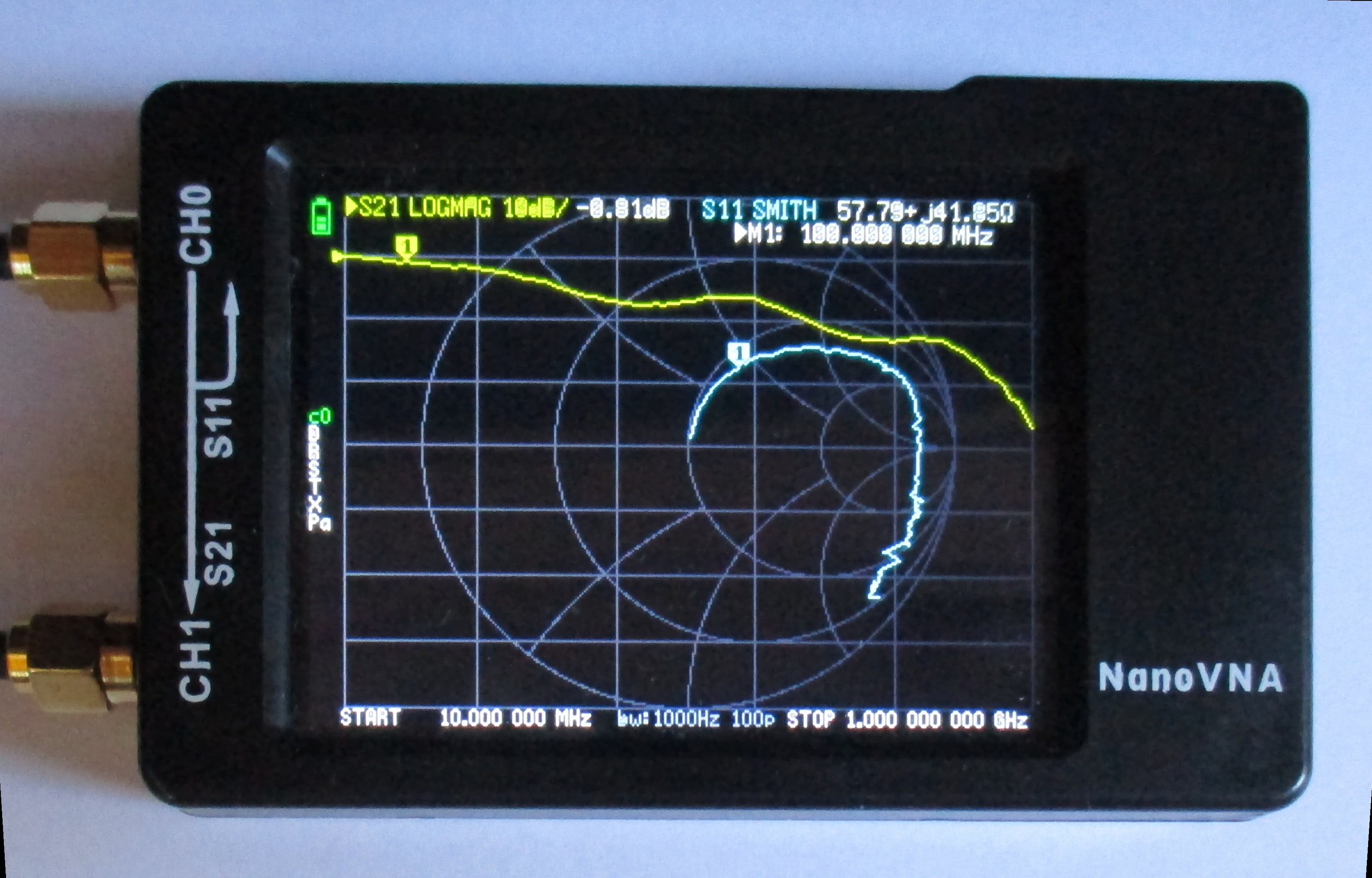
5.1 About this volume

The first four volumes of this dive built the NanoVNA as an instrument: what a reflection coefficient and an S-parameter actually are (Vol 1), the hardware lineages that turn that theory into a $100–1,500 handheld box (Vol 2), the OSL-and-through calibration discipline that makes any of its numbers trustworthy (Vol 3), and the S11/S21/Smith-chart/TDR measurement technique that reads the calibrated sweep back out (Vol 4). This volume is where all of that lands on an actual antenna at the top of a mast, a BALUN on the bench, and a purchase decision.

Unlike the antenna and matching-network dives this hub also covers, there is no DIY-build section here — you don’t build a NanoVNA, you use one. The equivalent structural section is the workflow: what an operator actually does with the instrument on deployment day, how to measure the matching hardware between the radio and the antenna, and what to load on a laptop once the on-device screen stops being enough. Section 2 walks the deployment-day sequence and gives a diagnostic tree for the single most common field complaint — “it isn’t matching” — that separates a length problem from a matching problem from a feedline problem from a common-mode problem, four failure modes with four different fixes that look identical on a bare SWR meter. Section 3 covers measuring BALUNs, ununs, and tuners, including the common-mode rejection test that verifies a choke is actually choking; it cross-links the BALUNs & UNUNs dive for the device theory rather than re-deriving it. Section 4 surveys the host-software and firmware landscape as it actually stands today, not as an older seed document remembers it. Section 5 is a dated buy survey across the price ladder the ecosystem now spans — considerably wider than the “$50–300” bracket this dive’s own project card still quotes. Section 6 is the highest-stakes content: the instrument’s real limits, sourced carefully enough to state a dynamic-range number without lying about what frequency it applies to. Section 7 closes out the gotchas and myths, and Section 8 hands off — this volume, and this whole five-volume dive.

One housekeeping note before any of that: every model designation, price, and specification in this volume was checked against a live vendor or manufacturer page, a project’s own GitHub repository, or a component manufacturer’s datasheet, as of late July 2026, and is marked accordingly below. Where a number could not be pinned to a live source this session — because a listing didn’t resolve, a vendor blocked the fetch, or no public specification exists — that is stated explicitly, with the best available reference point, rather than filled in from memory. This matters more in this volume than in most: the migrated seed material behind this dive quoted dynamic-range figures as flat numbers with no frequency attached, which is very close to a meaningless spec, and one purpose of Section 6 is to not repeat that mistake.

5.2 The deployment-day antenna workflow

A NanoVNA sweep is cheap enough to run constantly, and the discipline that separates a well-run deployment from a frustrating one is running it at the right moments, in the right place, and reading the right thing when it goes wrong.

5.2.1 Before you hoist

Three checks belong on the bench, before the antenna goes anywhere near its final position, because every one of them is far easier to fix on a table than forty feet up a mast.

Calibrate and verify the calibration, per Vol 3’s OSL-and-through discipline, at whatever reference plane you intend to use for the hoisted sweep — the antenna’s own feedpoint if you can reach it after deployment, or the shack end of the feedline if you can’t (Section 2.2 below is about exactly this choice). Verify the cal with a known-good load before trusting anything downstream of it; a bad calibration produces a plausible-looking but wrong sweep, and nothing in the rest of this workflow catches that on its own.

TDR the feedline before it goes up, not after. Vol 4’s time-domain-reflectometry technique finds a damaged shield, a bad crimp, or a kinked connector as a discrete reflection at a specific distance along the cable — and a feedline with an undetected fault, once it’s fastened along a mast and weatherproofed at both ends, is a much less pleasant thing to diagnose and repair than the same cable coiled on a bench. A clean TDR trace on the feedline alone, before the antenna is even connected, removes one whole branch of Section 2.4’s diagnostic tree before you’ve climbed anything.

Sweep the matching network in isolation if the build has one. A BALUN, unun, or tuner that will sit at the feedpoint is worth its own S21 characterization on the bench first (Section 3), against a resistive load matched to its rated output impedance, before it’s buried in a weatherproofed enclosure at the top of a mast. A choke that already shows poor common-mode rejection on the bench is not going to improve once it’s installed; catching that now is a five-minute fix instead of a return trip.

5.2.2 After you hoist — and at which end

Once the antenna is in its operating position, the workflow every earlier volume in this dive has been building toward finally runs: connect the calibrated NanoVNA, sweep the design band with margin on either side, and read where the minimum actually sits.

The one decision that changes what that sweep means is where you put the reference plane — at the antenna’s own feedpoint, or at the shack end of whatever feedline connects it to the operating position. The figure below makes the reason this matters concrete: a feedline has loss, and that loss attenuates the reflected wave twice, once on the way to the antenna and again on the way back. The standard transmission-line result is |Γ|_apparent = |Γ|_true × 10^(−A/10), where A is the line’s one-way loss in dB (so A = αL for a line of length L with loss α per unit length). The exponent is worth deriving rather than memorising, because it is easy to get a factor of two wrong in either direction: a one-way loss of A dB costs the amplitude a factor 10^(−A/20), the wave makes the trip twice, so the round-trip amplitude factor is 10^(−2A/20) = 10^(−A/10). Concretely, 3 dB of one-way feedline loss is 6 dB round trip, which scales |Γ| by 0.50 — not the 0.25 that a doubled exponent would imply — a real mismatch at the feedpoint looks smaller, and the SWR looks better, by the time it has traveled down a lossy line and back. A long run of RG-58 at 28 MHz, or any coax at all near the top of its rated frequency, can turn a feedpoint that would fail a strict return-loss target into a shack-end reading that looks comfortably matched.

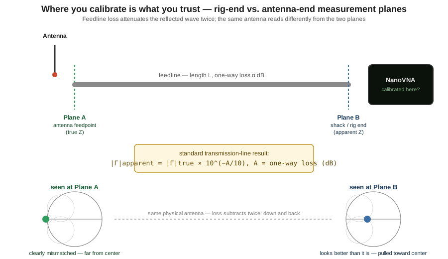
Neither plane is “wrong” — they are answering different questions. Calibrating at the feedpoint gives the antenna’s true impedance, which is what you want for trim decisions and for validating a model or a build. Calibrating at the shack end gives the number the transmitter actually sees, which is what matters for whether the rig’s output stage is happy — and it is also, unavoidably, the easier calibration to reach on a permanent installation with the feedpoint forty feet in the air. The workflow that gets this right is deliberate about which plane it’s reading at any given step: use the feedpoint plane while trimming an antenna to resonance, and don’t mistake a good shack-end reading through a long or lossy line for evidence that the feedpoint itself is clean.

5.2.3 What a good final sweep looks like

Independent of which antenna family is under test — the per-antenna volumes elsewhere in this hub each give their own target numbers for return loss, SWR floor, and bandwidth — a properly deployed and matched antenna shares three signatures on the NanoVNA screen: the S11 minimum sits within the intended trim tolerance of the design frequency; the Smith-chart marker at that minimum sits close to the real axis, reactance near zero; and — the check every antenna volume in this hub repeats for good reason — the reading does not move when you flex or reroute the feedline a meter or two below the feedpoint. That last one is the fingerprint of a clean common-mode situation, and it is cheap enough to run on every single sweep that there is no excuse for skipping it.

5.2.4 The “it isn’t matching” diagnostic tree

When the sweep doesn’t show that picture, the field question is always the same — “it isn’t matching” — but that one symptom hides at least four distinct causes with four distinct fixes, and treating the wrong one wastes a climb. Vol 4 already gave the raw fault-finding techniques (TDR distance-to-fault, Smith-chart pattern reading); the tree below is the decision sequence that applies them in the right order.

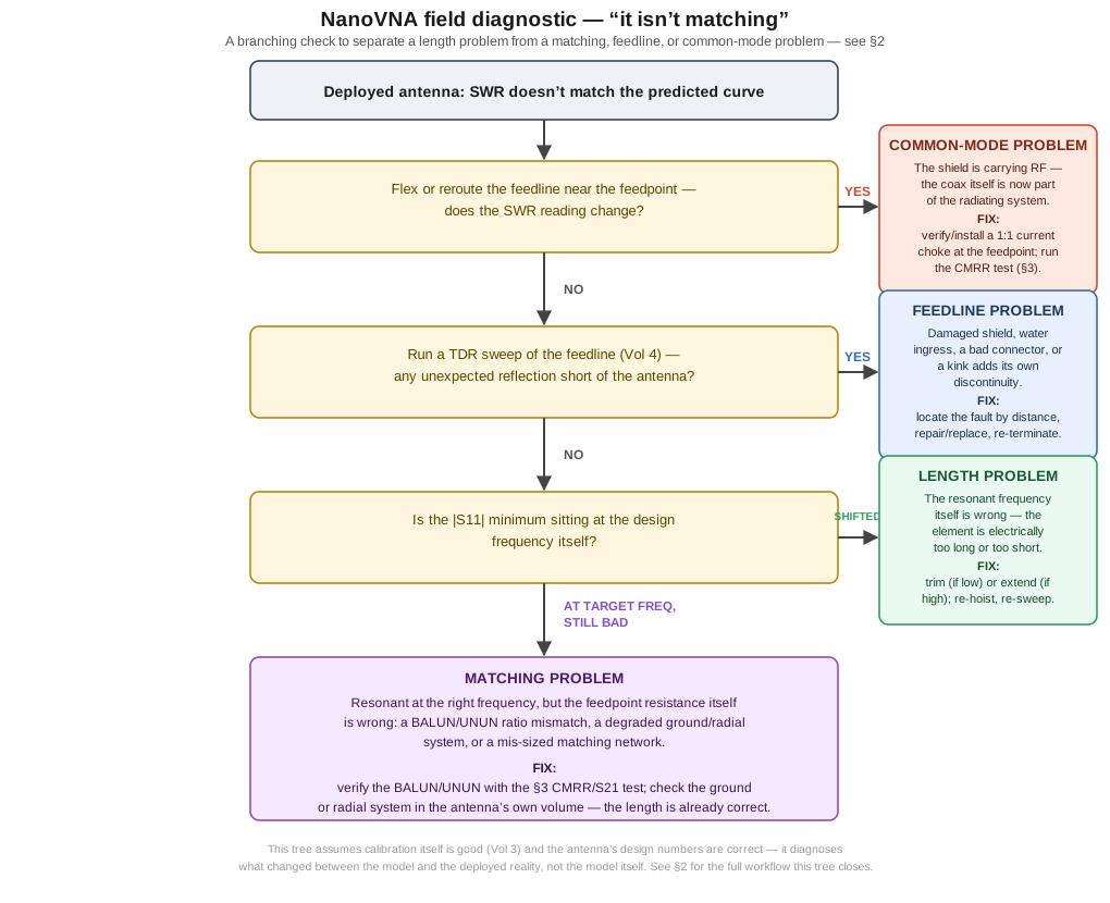
Read the tree in the order it’s drawn, because each check is cheaper than the next and each one rules out a whole failure class before you spend effort on the next question:

1. Flex the feedline near the feedpoint first. If the reading moves, stop — that is a common-mode problem, not a length or matching problem, and no amount of trimming fixes it. The fix is a working 1:1 current choke at the feedpoint, verified with Section 3’s test, not a longer or shorter element.

2. If the reading is stable under flexing, TDR the feedline. An unexpected reflection short of the antenna’s own distance means the feedline itself has a fault — the antenna and its matching network may be entirely correct and you are chasing a symptom the cable is causing.

3. If the feedline is clean, look at where the minimum sits. A minimum shifted off the design frequency, with an otherwise normal shape and depth, is a length problem: the element is electrically too long or too short, and the fix is exactly what the per-antenna trim workflows in this hub already describe.

4. If the minimum sits at the right frequency but the SWR still isn’t good there, the antenna’s resonant length is correct and the fault is in the matching itself — a BALUN or unun ratio that doesn’t fit the actual feedpoint impedance, a radial or ground system that hasn’t been given enough return-current capacity, or a mis-sized matching network. This is the case most often mistaken for a length problem, because the instinct on seeing bad SWR is to reach for the trim tool — but trimming a correctly-resonant antenna moves it off frequency without fixing the actual defect.

The tree assumes the calibration itself is trustworthy (Vol 3) and that the antenna’s design numbers are correct; what it diagnoses is what changed between the model and the deployed reality, which is nearly always one of these four things and rarely a fifth.

5.3 Measuring BALUNs, ununs and tuners

A BALUN, unun, or antenna tuner is a two-port device, and Vol 4’s S21 technique is the right tool for characterizing it — but the single most important thing to verify about a current-mode BALUN or unun is not its insertion loss, it’s whether it actually blocks common-mode current, and that needs its own test setup. The device theory behind why this matters — what a current BALUN is trying to accomplish, ferrite mix selection, turns-count and choking-impedance targets — belongs to the BALUNs & UNUNs dive and is not re-derived here; this section is purely the measurement technique.

5.3.1 Insertion loss and ratio verification

The straightforward S21 test — calibrate through, connect the DUT’s input to port 1 and its output (loaded with a resistor at the DUT’s rated output impedance) to port 2, and sweep — verifies that a BALUN or unun is passing power with the loss its datasheet claims, at the impedance ratio it claims. A 1:1 current BALUN loaded with 50 Ω should show a flat, low insertion loss across its rated range; a 9:1 unun loaded with a 450 Ω non-inductive resistor should show the same. This is exactly Vol 4’s general S21 workflow applied to matching hardware instead of a filter, and it catches a wound-wrong core, a cracked toroid, or a genuinely lossy design before it goes to the feedpoint.

For an antenna tuner, the same S21 measurement — with the tuner tuned for a 50 Ω match into a 50 Ω load, then swept — gives the tuner’s own insertion loss, which is the number that matters when deciding whether a tuner-fed compromise antenna is winning or losing against a resonant one; a lossy autotuner network can quietly eat more power than an equivalent-SWR mismatch would have cost without it.

5.3.2 The common-mode rejection test

Insertion loss says nothing about whether the choke is actually choking, and a BALUN can pass the S21 test cleanly while doing essentially nothing to block common-mode current on the shield. The rigorous way to measure this directly — a technique long established in the ham-radio ferrite-choke literature — treats the choke as an in-line common-mode impedance and reads it with a single-port measurement.

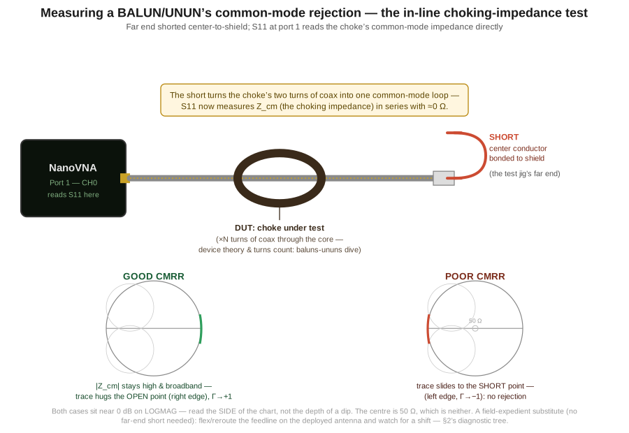
The setup: wind or install the choke on the length of coax it will actually be used with, connect one end to the NanoVNA’s port 1 through a calibrated reference plane, and at the far end short the center conductor to the shield. This turns the coax’s two conductors, in parallel, into a single loop as far as common-mode current is concerned — the differential-mode path is shorted out entirely, and the only thing left in series between port 1 and that near-zero-ohm short is the choke’s own common-mode impedance. The S11 measurement at port 1 is now, directly, the reflection off Z_cm in series with roughly 0 Ω — converting that S11 to impedance (the NanoVNA does this natively) reads the choking impedance across the swept band.

What good looks like: a high, broadband common-mode impedance shows up on the Smith chart as a trace hugging the open-circuit point at the extreme right edge — Γ → +1, per Vol 1’s convention — because a choke doing its job presents an impedance far above 50 Ω. A 1 kΩ common-mode impedance is Γ = +0.905; 5 kΩ is Γ = +0.980. What poor CMRR looks like: the trace slides to the left edge, toward the short-circuit point Γ → −1, because a choke that isn’t choking leaves the common-mode path looking like a low impedance — 5 Ω reads Γ = −0.818. The centre of the chart is neither of those things: it is 50 Ω, a matched load, which is not what either a good or a bad choke should produce.

A warning about the LOGMAG display specifically, because this is where the test is most often misread: both a good choke and a bad one sit close to 0 dB return loss. 1 kΩ reads −0.87 dB and 5 Ω reads −1.74 dB — a large mismatch either way, just in opposite directions. A deep notch on LOGMAG would mean a good 50 Ω match, which is the one thing a common-mode choke should never look like. If you find yourself hunting for a notch on this test you have confused it with the in-line S21 insertion-loss version, where a deep notch genuinely does mean high series attenuation. On this S11 test, read the side of the chart, not the depth of a dip. The specific ohm-value targets for a given core, mix, and turns count are the BALUNs & UNUNs dive’s territory; this test is how you find out whether a given real-world choke, on your bench, is hitting them.

The field-expedient substitute — useful once the choke is already installed at a feedpoint and a far-end short isn’t practical — is the flex-the-feedline check from Section 2.4: if the deployed antenna’s sweep changes noticeably when you grab and move the coax a meter or two below the choke, common-mode current is riding the shield regardless of what the choke’s datasheet claims, and the CMRR bench test above is the next diagnostic step once the antenna comes back down.

5.4 Host software — NanoVNA-Saver and the alternatives

The on-device screen is enough for a quick field check; a laptop connection buys larger plots, sweep logging and overlay, scripted automation, and file export — and the software landscape supporting that has moved since this dive’s seed material was written, so this section is checked directly against each project’s own repository rather than repeated from an older summary.

5.4.1 NanoVNA-Saver — still the default

NanoVNA-Saver remains the dominant cross-platform host application, and it is genuinely, actively maintained: its GitHub repository shows roughly 1,700 commits on the main branch, open pull requests and issues under active triage, and binary releases for Windows and Linux (development itself is primarily on Debian 11; macOS is supported as well). It’s GPLv3-licensed, free, and reads from the full range of NanoVNA-family hardware — the original NanoVNA-H/H4 lineage and the NanoVNA-F variants are explicitly supported. Its feature set covers multi-segment sweeps for extended resolution beyond a single device sweep’s point count, Touchstone (S1P/S2P) import and export for interchange with other RF software, in-application calibration management, several chart formats, and a TDR mode built on the same math Vol 4 covers on-device. For anyone doing more than a single quick field check, this is still the right first tool to reach for.

5.4.2 NanoVNA-App

NanoVNA-App, originally by Erik Kaashoek and actively carried forward in a fork maintained by DiSlord (the same developer behind the NanoVNA-D firmware discussed below), is a Windows-only C++ application distinct from NanoVNA-Saver’s Python codebase. It trades NanoVNA-Saver’s broader platform support for a smaller, more responsive footprint on Windows specifically — the tradeoff every NanoVNA-App user cites is faster redraw and lower memory use against a less polished UI and Windows-only availability. Its repository shows real, continuing activity, not an abandoned one-off.

5.4.3 Scriptable and specialized alternatives

For a reader building automated test benches rather than doing manual sweeps, NanoVNA-MATLAB (by the same author, qrp73, who also maintains a NanoVNA firmware modification) is a set of MATLAB scripts that connect directly to a NanoVNA, save S2P files, and display LogMag, Smith-chart, and TDR step-response views — a legitimate option for a reader who wants sweeps driven from a scripted environment rather than a GUI, and worth knowing about even though it has a much smaller user base than NanoVNA-Saver. One correction to the seed material behind this dive, and it is a correction of attribution, not of existence. An earlier draft of this hub’s reference notes cited “NanoVNA-QT by qrp-labs”. The attribution is wrong — qrp-labs (Hans Summers’ QRP kit company) has nothing to do with it — but NanoVNA-QT is a real and actively maintained project, hosted under the nanovna-v2 organisation, the same org that maintains the V2/S-A-A-2 firmware lineage discussed in §4.4. It is a C++/Qt5 cross-platform PC GUI (Linux, macOS, Windows) written specifically for the V2 series — the V2 Plus4 and Plus4 Pro — and NanoRFE advertise it directly as the native PC software for that hardware. That makes it directly relevant to this volume rather than a footnote: §5’s buy survey recommends exactly the V2 Plus4/Pro tier that NanoVNA-QT is the native host application for, so a reader buying into that tier should know its first-party software exists and is not NanoVNA-Saver.

5.4.4 The firmware question

Host software reads data the device’s own firmware produces, and which firmware is right depends entirely on which hardware family is in hand — the three architectural lineages Vol 2 covers in hardware terms have three separate firmware histories:

For the original NanoVNA-H/H4 lineage (edy555’s original design as carried forward by hugen79’s hardware revisions), the actively maintained community option is DiSlord’s NanoVNA-D firmware — a substantial fork adding SD-card support, an external serial connection, and faster measurement and host-exchange performance over the CPUs this hardware family uses (the per-model silicon is Vol 2’s territory). Its repository shows real ongoing activity and a genuine following (roughly 500 stars at last check), and it is the fork most H4-class owners flash in place of the stock factory firmware today.

For the V2 / S-A-A-2 architecture — the lineage sold today as the NanoVNA V2 Plus4 and V2 Plus4 Pro (Section 5) — firmware lives in a separate, actively developed repository targeting the V2.2, V2 Plus, and V2 Plus4 hardware variants specifically, with its own developer Discord and a vendor-hosted versions page as the canonical release channel. This is architecturally a different codebase from the H/H4 lineage’s firmware, not a variant of it — a point worth stating plainly because the seed material behind this dive asserted “all NanoVNAs run the same firmware” is false, and the real answer is more specific than that: there are at least three separate firmware lineages, one per hardware architecture, and flashing the wrong one is not an option the hardware even permits.

For the newest, highest tier — the NanoRFE-branded VNA6000 series (Section 5) — no public firmware repository could be located this session, which is itself worth noting rather than assuming: unlike the original NanoVNA’s fully open hardware-and-firmware lineage, this newer premium tier appears (though this could not be confirmed definitively) to be a more closed, single-vendor product, closer in that respect to a conventional commercial instrument than to the community-firmware tradition the rest of this family grew out of.

5.5 The buy survey — ranked, as of late July 2026

The instrument family covered by this dive has genuinely outgrown the “$50–300” bracket this project’s own scaffold notes still describe — the ecosystem has grown a real premium tier above that range, verified directly against live vendor listings this session. Every price and specification below was checked against the vendor’s own current product page; where a spec (most often dynamic range) is quoted by the vendor without a test frequency attached, that is noted explicitly rather than repeated as if it were a complete number — Section 6 explains why that omission matters.

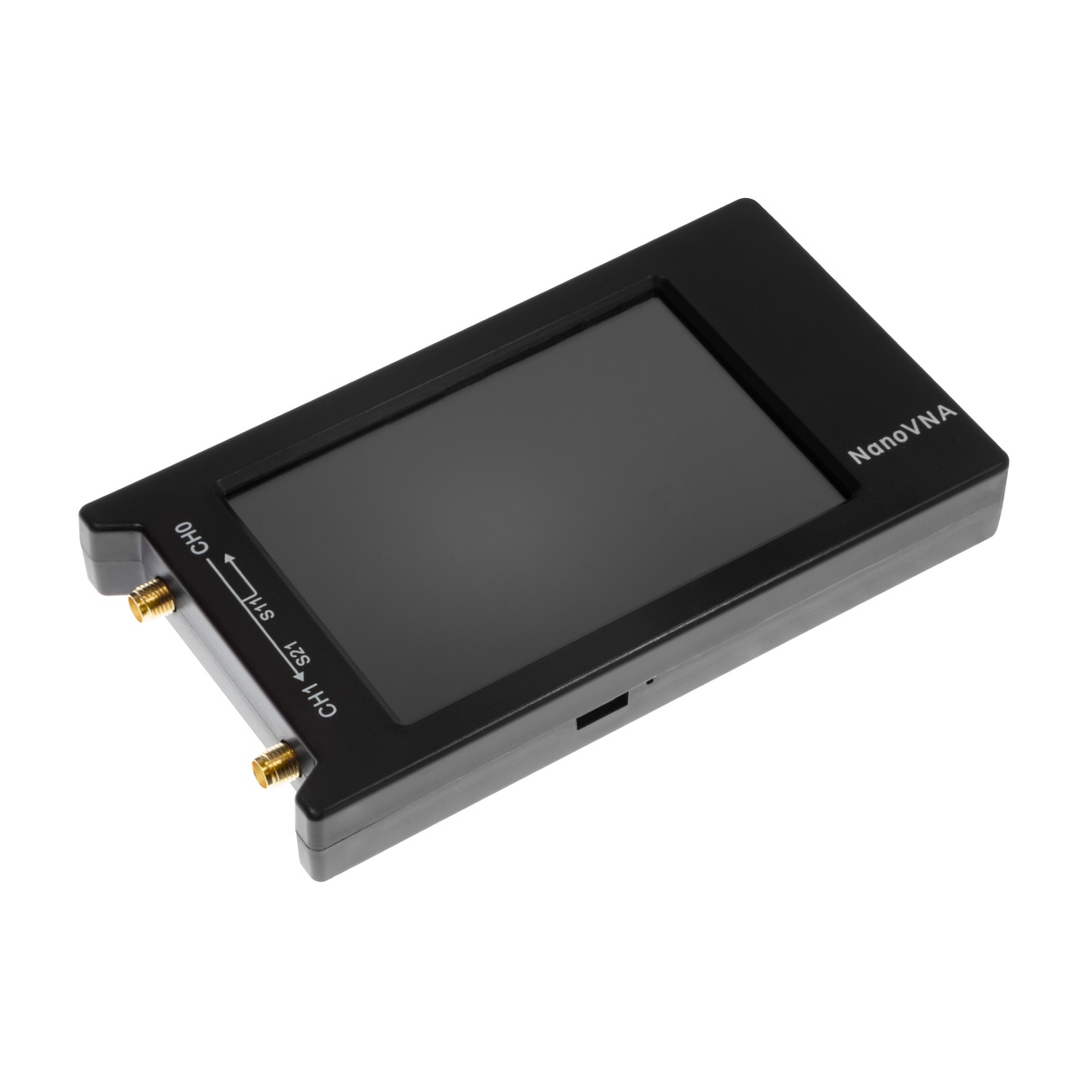
Table 1 — 5. The buy survey — ranked, as of late July 2026

Tier	Product	Frequency range	Dynamic range (as quoted)	Price (late July 2026)	Notes
Entry	NanoVNA (base model)	50 kHz – 900 MHz+	Not stated on this listing	$99.95 (verified, Nooelec)	2.8″ TFT touchscreen, includes a SOLT SMA calibration kit, two 30 cm test cables, USB-C cable, and a carrying case. The floor of the current market — a real, complete kit, not a bare board.
Entry+	NanoVNA Bundle	50 kHz – 900 MHz+	Not stated on this listing	$139.95 (verified, Nooelec)	Same base unit plus a 6-piece attenuator set, quick-connect adapters, and low-loss LMR200 test cables — the accessory-inclusive version of the entry unit above.
Mid	NanoVNA-H4	10 kHz – 1.5 GHz+	Not stated on this listing	$124.95 (verified, Nooelec)	4″ TFT touchscreen (the meaningful upgrade over the entry unit’s 2.8″), 0.5 ppm frequency accuracy, −13 dBm RF output, 1950 mAh battery, USB-C. The sweet-spot general-purpose unit — see Section 6.4 for what that fixed −13 dBm output does and doesn’t let you test.
Upper-mid	NanoVNA V2 Plus4 (S-A-A-2 architecture)	50 kHz – 4.4 GHz	90 dB (vendor spec; no test frequency stated — see §6.1)	$299 (verified, nanorfe.com)	A genuinely different architecture from the H4 lineage (Section 4.4), not a rebadge — higher rated frequency ceiling and rated dynamic range in the same size class.
Upper-mid+	NanoVNA V2 Plus4 Pro	50 kHz – 4.4 GHz	90 dB (vendor spec; no test frequency stated)	$399 (verified, nanorfe.com)	Same core hardware family as the Plus4, with adjustable IF bandwidth, better temperature stability, and reduced trace noise per the vendor’s own listing — a real, stated set of upgrades, not just a price bump.
Premium	NanoRFE VNA6000-A	50 kHz – 6 GHz	95 dB (vendor spec; no test frequency stated)	$789 (verified, nanorfe.com)	A distinctly newer, higher-tier product line than the traditional NanoVNA family, marketed explicitly around Wi-Fi 6 / 5.8 GHz ISM-band coverage. This is the point on the ladder where the instrument family starts overlapping the low end of the companion Analyzers & VNAs dive’s territory.
Top	NanoRFE VNA6000-B	50 kHz – 6 GHz	110 dB (vendor spec; no test frequency stated)	$1,499 (verified, nanorfe.com)	The vendor’s own flagship framing — “custom low-noise architecture,” “professional laboratory performance.” At this price and this dynamic-range claim, it is worth asking, before buying, whether the actual requirement is better served by a genuine entry-level bench VNA instead; see Section 6.5.

Two models this dive’s own seed material named could not be confirmed at a live listing this session. The LiteVNA-64 (historically the ~6.3 GHz, 70–80 dB premium consumer NanoVNA cited across this hub’s other volumes) and the NanoVNA-F V3 (the non-touch, 5″-screen tabletop variant) both failed to resolve at every vendor page attempted this session — a Tindie listing returned a bot-blocking 403, a UK VNA specialty retailer returned repeated server errors, and no public repository for the LiteVNA-64’s designer turned up a current sales channel. That is not the same as confirming they’re discontinued — Chinese-market resellers for hardware in this space frequently exist outside the retailers this session could reach — but it means the ~$200–300 figures other volumes in this hub cite for these two models should be treated as last known, not currently re-verified, and a buyer should expect to re-check availability directly before ordering either one.

Reading the ladder. Compared to the “$50–300” bracket this project’s own earlier notes describe, the ecosystem has grown a real premium tier well above that range — the VNA6000-B’s $1,499 asking price and 6 GHz coverage sit closer to an entry-level lab instrument than a hobbyist gadget. For most amateur antenna, BALUN, and feedline work at HF through low UHF, the $124.95 NanoVNA-H4 remains the practical sweet spot this dive has assumed throughout its antenna-volume cross-links. The V2 Plus4 tier earns its higher price with a genuinely different, wider-bandwidth architecture, not just a bigger screen; the VNA6000 tier is worth its premium only when the actual need — 6 GHz coverage, or a dynamic-range floor deep enough to matter — is real. Section 6 is where to check that before spending $789–1,499 on a claim this session couldn’t verify with a frequency attached.

What to avoid. An unqualified dynamic-range figure, of the kind every model in the upper half of this table quotes, isn’t disqualifying on its own — Section 6.1 explains why every consumer VNA in this class shares that marketing habit — but a listing pairing an unqualified DR number with an unusually aggressive price (a “6 GHz, 120 dB” board under $200, say) is worth real skepticism; no vendor checked this session offered that combination, and one that does should be treated as a claim to verify, not a bargain to trust.

5.6 The instrument’s real limits

This is the section most worth getting right and most damaging if it’s wrong, because a dynamic-range number without a frequency attached to it — which is exactly what every current vendor listing in Section 5 provides — is close to meaningless, and the discipline this section holds itself to is quoting only what a live source actually states, with the frequency it was stated at, rather than smoothing that gap over with an invented curve.

5.6.1 Dynamic range — and at what frequency

The vendor habit of quoting a flat dynamic-range number is a real, observable problem, not a hypothetical one. Every current listing checked in Section 5 — the V2 Plus4’s 90 dB, the V2 Plus4 Pro’s 90 dB, the VNA6000-A’s 95 dB, the VNA6000-B’s 110 dB — states the figure with no test frequency attached. A dynamic range spec without a frequency tells you almost nothing about where in the swept band that number actually holds, because every architecture in this family loses dynamic range as frequency rises: the source’s available power rolls off, receiver noise figure typically worsens, and — for architectures that reach their top frequency via harmonic generation rather than a fundamental synthesizer — the harmonic content driving the mixer gets weaker at each successive multiple.

The one figure this session found stated with an explicit frequency qualifier comes from the technical documentation in hugen79’s own NanoVNA-H firmware repository, for the original NanoVNA-H/H4 architecture specifically: it states that the 50 kHz–300 MHz range, covered by the Si5351 synthesizer’s direct (non-harmonic) output, provides better than 70 dB of dynamic range. That is a genuinely useful number precisely because it comes with a boundary attached — it is a claim about the bottom third of the H4’s rated 1.5 GHz+ range, the portion reached without resorting to harmonic mixing. Above 300 MHz, this same hardware reaches its rated upper frequency by using higher odd harmonics of the same Si5351 clock — a well-understood RF technique (harmonic sampling / harmonic-mixer receivers), and one that inherently delivers less power, and therefore a worse noise floor and reduced dynamic range, at each higher harmonic. Three further frequency-qualified figures were sourced elsewhere in this dive, and together with the 70 dB number they are enough to describe the shape of the problem without inventing a curve. From nanovna.com’s own documentation: a well-fabricated original unit reaches about 40 dB at 900 MHz, and the improved NanoVNA-H rev3.4 and later, and the H4, hold roughly 40 dB out to 1.5 GHz — both squarely in the harmonic-extended region, and both showing the same thing, that reaching above the Si5351’s fundamental range costs on the order of 30 dB. From NanoRFE’s own product pages, the fundamental-only V2 Plus4 and Plus4 Pro are specified at 90 dB and 96 dB respectively, explicitly at 1 GHz with AVG=20 — a condition worth quoting in full, because averaging is doing real work in that number and a figure without it is not comparable. Vol 2 sets those out family by family with the architectural reason behind each. What is still genuinely unsourced is any frequency-qualified figure for the VNA6000 line, whose 95–110 dB claims carry no stated test condition — that gap is real and is stated here rather than papered over.

What can be said with confidence, as general RF engineering reasoning rather than a sourced measurement: dynamic range on every architecture in this family is highest toward the low end of its rated range and degrades toward the top, and an architecture reaching its top frequency by harmonic multiplication (the traditional NanoVNA-H/H4 lineage above 300 MHz) should be expected to degrade faster than one using a fundamental wideband synthesizer across its whole range (the general design approach community discussion attributes to the V2/S-A-A-2 architecture, though this session could not independently confirm the specific claim with a vendor-published curve). Practically: trust a vendor’s single flat dynamic-range number the least at the top of that device’s rated frequency range, and treat any of Section 5’s unqualified 90–110 dB figures as an upper bound reachable somewhere in the swept band, not a number you can assume holds uniformly from 50 kHz to the rated ceiling.

5.6.2 Calibration drift in the field

Vol 3 owns the calibration procedure itself; the field-relevant point here is narrower: a calibration taken on the bench does not necessarily hold once the instrument, the cables, and the connectors experience a different temperature, and none of the vendor pages checked for this volume publish a temperature-drift specification for their instruments — a genuine absence worth stating rather than papering over with an invented coefficient. The practical discipline this dive’s earlier volumes already establish (re-calibrate at the start of each measurement session, verify against a known load before trusting a sweep) is the right response to an unquantified risk: rather than trying to correct for a drift number nobody publishes, the workflow avoids depending on one by re-verifying cheaply and often. A bench calibration taken indoors at 20 °C and carried unverified to a rooftop sweep in July sun is the specific case worth calling out — the temperature swing between those two conditions is large enough that re-verifying against the load standard before trusting the rooftop sweep costs thirty seconds and removes the whole question.

5.6.3 Microwave-end performance

Every model in Section 5’s table is rated to a specific top frequency — 900 MHz, 1.5 GHz, 4.4 GHz, or 6 GHz — and, consistent with Section 6.1’s general point, accuracy and dynamic range are their weakest right at that ceiling on every architecture in this family. This session found no vendor-published accuracy-versus-frequency curve for any model in the table, which is itself the honest finding: unlike a calibrated lab VNA, whose datasheet typically states measurement uncertainty as an explicit function of frequency, none of the consumer-tier vendors checked here publish that curve for their instruments. The practical implication is the same one Vol 3’s calibration-slot discipline already assumes: calibrate as close as possible to the actual frequency range you intend to measure, don’t extrapolate a calibration taken at HF to a microwave-band measurement, and treat a sweep taken within the last 10–15% of a device’s rated range with the most skepticism it’s due — that is exactly the region no vendor in this survey is willing to publish a number for.

5.6.4 Stimulus power, phase noise, and stability

The one hard number this session could verify directly on this topic is the NanoVNA-H4’s rated RF output power of −13 dBm, fixed, per its own manufacturer listing — the instrument’s source is not adjustable across a swept power range, which means it cannot characterize a DUT’s power-dependent behavior (amplifier compression, PIN-diode switching thresholds, any nonlinearity that only shows up at higher drive levels). This is a genuine, verifiable limit distinct from dynamic range, and it is one of the clean handoff triggers to a real signal-generator-driven VNA setup (Section 6.5).

On phase noise and frequency stability specifically, this session could not locate a vendor-published specification for any model in Section 5’s table, and did not find a live datasheet for the clock-generator component the original architecture is built around (a general-purpose I2C-programmable clock synthesizer, not a purpose-built low-phase-noise RF source) to cite a specific jitter figure. What can be said honestly: a general-purpose clock synthesizer of the kind these low-cost architectures use is, by the nature of that class of part, not designed to the same phase-noise specification as a dedicated RF synthesizer in a lab-grade VNA, and the community consensus reflected across the NanoVNA firmware repositories checked for this volume treats phase stability as a known, accepted tradeoff of the platform’s price point rather than a specification anyone publishes a number for. Treat this as a real limitation whose exact magnitude this volume declines to state numerically, having found no source that states it either.

5.6.5 The honest handoff to a real VNA

Four cases in this family’s actual use come up often enough to name plainly, and all four point to the Analyzers & VNAs dive rather than to a bigger NanoVNA:

• Deep stopband or high-isolation characterization — verifying a filter’s rejection, or a coupler’s isolation, meaningfully below the dynamic-range floor discussed in Section 6.1 needs an instrument with a published, frequency-qualified dynamic range deep enough to trust the number, not an instrument whose vendor won’t state one.
• Swept-power or compression testing — Section 6.4’s fixed-output-power limitation is architectural, not a firmware gap; testing DUT behavior across a power range needs a source that can sweep power, which nothing in this family’s current lineup does.
• Traceable, certified calibration — compliance or lab work that needs a calibration with a paper trail back to a national standard is not something any instrument in Section 5’s table, or its included calibration kit, is built to provide.
• Frequencies above roughly 6 GHz, or work anywhere near the top of whatever ceiling the specific model in hand is rated to, per Section 6.3’s accuracy caveat.

None of these four is a knock on the instrument family this dive covers — they are simply outside what a $100–1,500 handheld analyzer is built to do, and knowing which of the four applies before reaching for a bigger toy is the entire point of stating the limits this plainly.

5.7 Gotchas and myths

“Dynamic range is a single number” is Section 6.1 restated as a myth: every current vendor listing surveyed in Section 5 states dynamic range with no frequency attached, and the one figure this dive could source with a frequency qualifier (70 dB, but only up to 300 MHz on the original H/H4 architecture) applies to a fraction of any given model’s rated range. Quoting “90 dB” or “110 dB” without asking where in the sweep that holds is trusting an incomplete number.

“All NanoVNAs run the same firmware” is false, and more specifically false than that framing suggests: this dive found at least three separate, architecturally distinct firmware lineages currently active — DiSlord’s NanoVNA-D for the original H/H4 hardware, a separate repository for the V2/S-A-A-2 architecture with its own developer community, and (as best this session could determine) closed, vendor-specific firmware for the newer VNA6000 tier. Flashing firmware across these families isn’t a compatibility inconvenience — the hardware architectures underneath them are different enough that it isn’t an option at all.

“I calibrated last week, no need to re-cal” ignores that neither this volume nor any vendor page checked for it could find a published temperature-drift specification for these instruments — which is precisely the argument for re-calibrating at the start of every session rather than trying to reason about how much a week-old, unquantified drift has cost you.

“My rig shows 1.0:1, so the antenna is perfect” is Section 2.2’s measurement-plane distinction restated as a trap: a shack-end reading through a lossy or long feedline can look better than the true feedpoint impedance by exactly the two-way attenuation Section 2.2 derives, and the number worth trusting for a trim decision is the one read at, or as close as practical to, the feedpoint itself.

“A good S21 through a BALUN means it’s doing its job” conflates insertion loss with common-mode rejection — Section 3 is built entirely around the fact that these are two different measurements, and a BALUN that passes power cleanly can still do essentially nothing to stop common-mode current on the shield. Run the choking-impedance test, not just the insertion-loss test.

“NanoVNA-Saver is required for serious work” overstates the case in the opposite direction from the myth above: the on-device screen and the workflow in Section 2 are entirely adequate for a field deployment check. NanoVNA-Saver earns its place for logging, overlay comparisons, and file export — genuinely useful, not strictly necessary for a single sweep-and-trim session.

“The premium tier is always worth it, and the coax never matters” bundles two related overreaches. A $1,499 instrument whose vendor won’t state a frequency for its 110 dB claim is not automatically a better antenna-work tool than the $124.95 unit this dive cross-links from every antenna volume in this hub — the premium tier earns its price on genuine bandwidth and architecture upgrades, not a bigger unqualified spec number. And “the coax doesn’t matter” is only true for a short, low-loss HF run: the higher the frequency and the longer or lossier the line, the more a shack-end reading diverges from the true feedpoint impedance, which is exactly Section 2.2’s measurement-plane trap.

5.8 Where this volume — and this dive — hands off

This volume closed the NanoVNA dive by putting the first four volumes’ theory and technique to work: a deployment-day workflow that runs the right sweep at the right moment and reads a single ambiguous symptom — “it isn’t matching” — down a decision tree that ends in one of four distinct, correctly-targeted fixes; a rigorous common-mode rejection test for the BALUNs, ununs, and tuners every antenna volume in this hub eventually cites; a host-software and firmware landscape checked directly against each project’s own current repository rather than repeated from an aging summary, including a correction to a piece of seed material that named a software project this session could not confirm exists; a buy survey that found the instrument family has genuinely outgrown its original “$50–300” bracket, verified up through a $1,499 near-lab-grade tier; and — the section this volume treated with the most care — an honest account of the instrument’s real limits, stating one frequency-qualified dynamic-range figure this dive could actually source and declining to invent the rest of that curve.

Zooming out, this volume is also the last of the five that make up the NanoVNA dive. Vol 1 fixed the theory — reflection coefficients, S-parameters, and what a 2-port measurement is actually telling you. Vol 2 surveyed the hardware lineages this volume’s buy survey priced out. Vol 3 established the calibration discipline every measurement in this volume depends on being correct. Vol 4 built the S11/S21/Smith-chart/TDR measurement technique this volume’s workflow applies in the field and on the bench. And this volume closed the loop: theory, hardware, calibration, and technique, put to work on an actual deployment.

The NanoVNA is the measurement instrument the rest of this Antennas hub leans on constantly — every antenna build’s tuning loop, every matching-network characterization, every feedline fault hunt in this hub cross-links back to some piece of this five-volume dive. The device theory behind the BALUNs, ununs, and tuners this volume measured lives in the BALUNs & UNUNs dive, cited here rather than reproduced. The instruments that pick up where this one’s limits (Section 6) end — deeper dynamic range, traceable calibration, swept power, microwave coverage past 6 GHz — live in the Analyzers & VNAs dive. And the transmission-line theory behind why a feedline’s loss changes what Section 2.2’s two measurement planes each read lives in the foundational transmission-lines & feedlines volume, cited rather than re-derived. This volume points to all three rather than duplicating them, consistent with the whole hub’s cross-linking discipline.

5.9 Resources

• NanoVNA-Saver — https://github.com/NanoVNA-Saver/nanovna-saver — the source verified for its active-maintenance status, license (GPLv3), supported hardware, and feature set in Section 4.
• DiSlord’s NanoVNA-D firmware — https://github.com/DiSlord/NanoVNA-D — the source verified for its hardware targets and activity level in Section 4.4.
• hugen79’s NanoVNA-H firmware repository — https://github.com/hugen79/NanoVNA-H — the source for the one frequency-qualified dynamic-range figure this dive could confirm (better than 70 dB, 50 kHz–300 MHz, direct Si5351 output) in Section 6.1.
• nanovna-v2/NanoVNA2-firmware — https://github.com/nanovna-v2/NanoVNA2-firmware — the source verified for the V2/S-A-A-2 architecture’s separate firmware lineage in Section 4.4.
• DiSlord’s GitHub profile — https://github.com/DiSlord — the source verified for the NanoVNA-App (forked from Erik Kaashoek’s original) listing in Section 4.2.
• qrp73’s GitHub profile — https://github.com/qrp73 — the source verified for NanoVNA-Q and NanoVNA-MATLAB.
• nanovna-v2/NanoVNA-QT — https://github.com/nanovna-v2/NanoVNA-QT — the real home of NanoVNA-QT, the Qt5 host application for the V2 Plus4 / Plus4 Pro, and the basis for §4.3’s correction of the seed material’s “by qrp-labs” attribution (the project itself is genuine).
• Nooelec — https://www.nooelec.com — the source verified for the base NanoVNA, NanoVNA Bundle, and NanoVNA-H4 prices and specifications in Section 5, including the −13 dBm fixed output figure used in Section 6.4.
• nanorfe.com — https://nanorfe.com — the source verified for the NanoVNA V2 Plus4, V2 Plus4 Pro, and NanoRFE VNA6000-A/B prices and vendor-quoted specifications in Section 5.
• The BALUNs & UNUNs dive — https://antennas.fubsypoly.com/baluns-ununs/vol-1/ — the device theory, ferrite mix selection, and choking-impedance targets behind Section 3’s measurement technique.
• The Analyzers & VNAs dive — https://antennas.fubsypoly.com/analyzers-vnas/vol-1/ — the instrument class this volume hands off to in Section 6.5 for the cases a NanoVNA genuinely isn’t built for.
• The hub’s foundational transmission-lines & feedlines volume — the coax-loss theory behind Section 2.2’s rig-end-vs-antenna-end measurement-plane distinction.