Finding the Load, and Matching by Hand

---

4.1 About this volume

Vol 3 ended on a problem it could not solve. The variable that decides your tuner’s loss is the load, not the SWR — the same 5:1 reading costs 0.20 dB into 250 Ω and 0.98 dB into 10 Ω — and nothing at the operating position tells you which of those you have. This volume is about finding out, and about what to do once you know.

That splits into three parts. Measuring the load is a twenty-minute job with a VNA and a handful of rules about where to stand, which is §2. Reading the result is the Smith chart, which §3 has to rebuild from scratch because the previous edition’s description of it was wrong in every line. And acting on it is §4 and §5: an L-network is exactly two moves on that chart, there are generally four ways to make them, and they are not equivalent.

Two findings deserve stating at the top.

The first is that this chapter’s Smith-chart section contains the same error as its schematics, stated independently. Vol 2 found the two L-network drawings wired with the shunt element on the wrong side, producing 5.33:1 and 6.45:1 from equations that were exactly right. §4 here finds that the chapter’s matching procedure prescribes the moves in the same wrong order, for both cases — and does so two paragraphs after stating the correct rule. That makes it a consistent misunderstanding appearing in two independent places rather than a drawing slip, which is a more serious diagnosis and a more useful one.

The second is a practical result I have not seen stated plainly. §5 enumerates all four L-networks that match one load and finds the two that use no inductor at all lose five to eight times less than the two that do. A load with reactance of the right sign supplies one of the network’s two reactances for free, and what is left can be built entirely from capacitors — whose Q at HF is an order of magnitude better than any roller inductor’s. When the load’s reactance allows it, the lowest-loss tuner setting is the one with the coil out of circuit, and it is invisible from the front panel.

4.2 Measuring the load, and where to stand

The instrument is a vector network analyser, and for this job the cheapest one will do — the NanoVNA dive covers what these instruments actually measure and its Vol 3 covers calibration, which is the part that matters here. What that dive does not cover is where in an antenna system to point it, which is a question with one right answer and several tempting wrong ones.

Measure at the terminals the tuner will connect to. Not at the antenna feedpoint. The tuner is handed whatever the feedline delivers, and Vol 1 §3 showed how completely a feedline can transform an impedance: an antenna presenting 26 − j420 arrived at the tuner as 8.77 − j2.78. If the tuner lives in the shack, walk the VNA to the shack and measure at the end of the coax that will plug into it. If you are choosing a remote tuner, measure at the feedpoint instead. The two measurements are of different things and neither substitutes for the other.

Calibrate at that plane. An open-short-load calibration performed at the VNA’s own connector measures the cable plus the antenna. Performed at the far end of the cable — the end that will meet the tuner — it measures what the tuner sees. That is the whole reason calibration standards exist, and getting it wrong is the most common way to produce a confident and useless number.

Expect the answer to move. The impedance at the tuner’s terminals is a property of the antenna and the feedline and the frequency. Change any of them and it changes. This is not a defect in the measurement; §6 turns it into a design freedom.

Do not measure through the tuner. A VNA looking into a tuner’s input sees the tuner’s current setting, which is the thing you are trying to choose. Disconnect it and measure the load directly.

Watch for common-mode current. If the feedline’s outer surface is carrying current, the impedance you measure will shift when you move the cable or touch it — and it will keep shifting after you have set the tuner. That is a symptom, not noise. The BALUNs and UNUNs dive covers the choke that fixes it; the diagnostic is simply to grasp the coax a quarter-wavelength back and watch whether the reading moves.

And never transmit into the analyser. A NanoVNA’s front end survives milliwatts. Disconnect it before the first tune-up, every time, including the time you are sure you remembered.

What you get for that effort is a complex impedance at each frequency you care about — and with it, the answer Vol 3 needed. A load of 250 Ω and a load of 10 Ω read identically on an SWR meter and sit on opposite sides of the loss curve. One measurement separates them.

4.3 The chart, described correctly

The Smith chart is the standard way of displaying that measurement, and it is worth understanding rather than merely reading, because its geometry is the geometry of matching networks. Unfortunately the previous edition’s account of it was wrong in essentially every line, so this section rebuilds it.

The chart is a plot of the reflection coefficient

Γ = (z − 1) / (z + 1)

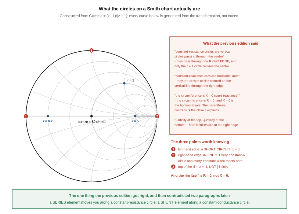
where z = Z / 50 is the impedance normalised to the reference. Every possible passive impedance maps somewhere inside the unit circle. The lead figure is constructed from that formula rather than traced, which is worth saying because it means the curves in it cannot be wrong in the way a sketch can.

From the transformation, two families of curves follow directly:

• Constant-resistance circles. A locus of constant r maps to a circle centred at (r/(1+r), 0) with radius 1/(1+r). Every one of them passes through Γ = +1, the right-hand edge. The r = 1 circle is the only one that also passes through the centre, and it does so because its centre is at 0.5 with radius 0.5.
• Constant-reactance arcs. A locus of constant x maps to a circle centred at (1, 1/x) with radius 1/|x|, clipped to the part inside the unit circle. These also all pass through Γ = +1.

And three points anchor the whole picture:

• The centre is 50 Ω — z = 1, Γ = 0, no reflection.
• The right-hand edge is infinity — an open circuit, where every constant-R circle and every constant-X arc converges.
• The left-hand edge is a short circuit — z = 0.
• The rim is R = 0: zero resistance, pure reactance, all the way round. The top of the rim is z = j1, which at a 50 Ω reference is +j50 Ω — an ordinary inductive reactance, not an infinity.

4.3.1 What the previous edition said

Set against that, the five claims in the chapter’s “Smith chart in 30 seconds”:

Table 1 — Set against that, the five claims in the chapter's "Smith chart in 30 seconds"

what it said	what is true
”the horizontal axis is pure resistance (X = 0)“	correct
”the centre point is 50 Ω”	correct
”constant-resistance circles are vertical circles passing through the centre”	they pass through the right-hand edge; only r = 1 crosses the centre, and “vertical circles” describes nothing
”constant-reactance arcs are horizontal arcs passing through the right edge”	the right edge is right; they are arcs of circles centred on the vertical line through that edge, not horizontal
”the circumference is X = 0 (pure reactance, at j∞ at the top, −j∞ at the bottom)“	the circumference is R = 0. The parenthesis contradicts the claim it explains — X = 0 is pure resistance. And both infinities are at the right-hand edge, not top and bottom

That is three of five wrong, one of them self-contradicting inside its own sentence.

⭐ And then the very next paragraph gets it exactly right: “Adding series reactance moves the impedance point along a constant-resistance circle. Adding shunt reactance (admittance) moves it along a constant-conductance circle.” Both halves of that are correct, and they are the only two facts you actually need to design an L-network. The chapter had the load-bearing sentence and surrounded it with a broken description of the chart it applies to.

4.4 An L-network is two moves

Here is the whole of L-network design, and it takes one paragraph once the chart is right.

A series element moves you along a constant-resistance circle. A shunt element moves you along a constant-conductance circle. To reach the centre you need to arrive on a curve that passes through it, and exactly two do: the r = 1 circle and the g = 1 circle. So: make one move to land on one of those two circles, then make the other kind of move to slide along it to the centre. Two moves, two elements, done.

Which circle you can reach determines which move comes first:

• If you can reach the r = 1 circle by a shunt move, do that, then finish with a series element. This works when the load lies outside the g = 1 circle — equivalently, when its conductance is at most 1/50 siemens.
• If you can reach the g = 1 circle by a series move, do that, then finish with a shunt element. This works when the load lies outside the r = 1 circle — equivalently, when its resistance is at most 50 Ω.

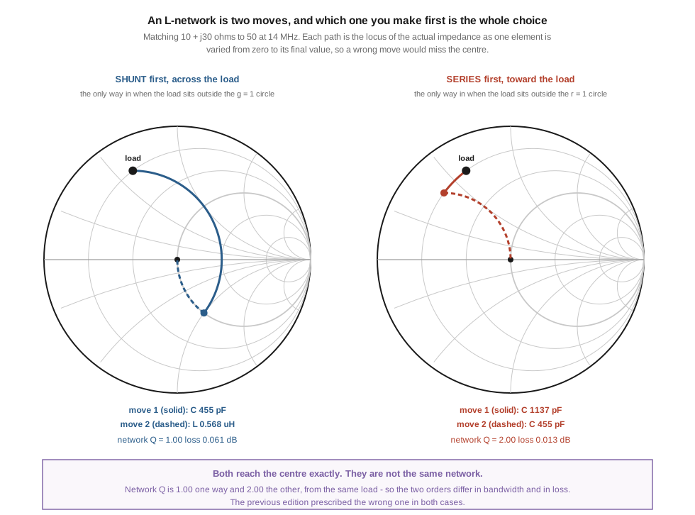
The figure matches 10 + j30 Ω to 50 Ω at 14 MHz. Its normalised resistance is 0.2 and its normalised conductance is 0.5, so it is outside both circles and both routes are open. Each path is drawn as the locus of the actual impedance as one element is swept from zero to its final value — so if a move were prescribed wrongly, the path would visibly miss the centre.

4.4.1 The procedure the previous edition gave

Against that, the chapter’s Step 3:

Step 3a (L-up): From the antenna point, trace along the constant-resistance circle until you reach the 50 Ω resistance circle.

Step 3b (L-down): From the antenna point, trace along the constant-conductance circle until you reach the 50 Ω conductance circle.

Both are impossible as written, and impossible for the same reason. Moving along your own constant-resistance circle keeps your resistance constant, so if you did not start on the r = 1 circle you will never arrive on it. Likewise for constant-conductance. Each step instructs the reader to travel along a curve that by definition cannot take them where they are going.

The roles are swapped. For a high-resistance load the first move must be the shunt one; for a low-resistance load it must be the series one. Step 3a has the series element first and Step 3b has the shunt element first, which is exactly backwards in both cases.

⭐⭐ This is the same inversion as the schematics in Vol 2, arrived at independently, two paragraphs after the chapter states the correct rule. That matters for how the rest of the chapter should be read. A single backwards drawing is a slip. The same error in the drawings and in the procedure, on both configurations, with the correct rule sitting between them, is a consistent misunderstanding — and it means the chapter’s other design guidance deserves computing rather than trusting. Every schematic and every procedure in this dive has been evaluated as drawn for that reason.

4.5 Four solutions, and why they are not equivalent

Each of the two routes has two variants, because the intersection with the target circle happens at two points — one above the axis and one below. So a load outside both circles admits four L-networks, all exact. For 10 + j30 Ω at 14 MHz, with an inductor of Q = 100 and capacitors of Q = 1000:

Table 2 — Each of the two routes has two variants, because the intersection with the target circle happens at two points — one above the axis and one below. So a load outside both circles admits four L-networks, all exact. For 10 + j30 Ω at 14 MHz, with an inductor of Q = 100 and capacitors of Q = 1000

first move	shunt element	series element	network Q	loss
shunt	C 227 pF	C 227 pF	1.00	0.013 dB
shunt	C 455 pF	L 0.568 µH	1.00	0.061 dB
series	C 455 pF	C 1137 pF	2.00	0.013 dB
series	L 0.284 µH	C 227 pF	2.00	0.107 dB

Every row presents 50.000 + j0.000 Ω. Two things separate them.

The two routes have different network Q — 1.00 for the shunt-first pair and 2.00 for the series-first pair. Vol 2 §3 established that Q is forced for a resistive load, and this is the qualification: when the load carries reactance of its own, the two routes make different use of it, and the resulting networks differ in bandwidth. The lower-Q route is the broader one and the one to prefer if you want a setting that survives moving a few tens of kilohertz.

⭐⭐ And the rows with no inductor lose five to eight times less than the rows with one. That is the finding worth carrying. The load here is inductive, and an inductive load already supplies part of what a matching network would otherwise have to provide — so two of the four solutions need only capacitors. Since a good air variable’s Q at HF runs in the thousands while a roller inductor’s runs from about 20 to 100, removing the coil from the circuit removes almost all of the loss with it.

Stated as a rule: when the load’s reactance has the sign the network wants, take the solution that leaves the coil out. The saving is larger than anything else available at the operating position, and it is completely invisible on an SWR meter — which is Vol 2’s degree-of-freedom problem and Vol 3’s wrong-variable problem meeting in one place.

4.5.1 How many solutions a load gets, and why an L-network can match anything

The count is not arbitrary, and working it out settles a question the previous edition raised and did not answer.

A load is inside the r = 1 circle when R > 50, and inside the g = 1 circle when G > 1/50. Can it be inside both? That would need R > 50 and X² < 50R − R² — and for any R above 50 the right-hand side is negative, so the second condition is unsatisfiable. No load is inside both. Geometrically the two circles span Γ from 0 to 1 and from −1 to 0 respectively, touching only at the origin.

That gives a complete map:

Table 3 — That gives a complete map

where the load sits	example	solutions
outside both circles	10 + j30 (r 0.20, g 0.50)	4
inside the r = 1 circle	250 + j0 (r 5.00, g 0.20)	2, shunt-first only
inside the g = 1 circle	8.77 − j2.78 (r 0.18, g 5.18)	2, series-first only

⭐ And since no load can be inside both, every load has at least one route to the centre: an ideal L-network can match anything. The L-network’s real-world limitation, which Vol 2 §6 quantified as a span of 52 Ω to 9.6 kΩ, is entirely about component values — the reactances the two circles demand simply become unbuildable at the extremes. The topology is not the constraint; the parts bin is.

4.5.2 Bandwidth does not simply follow network Q

One more result, and it qualifies something from Vol 2. Sweeping each of the four networks with the load held fixed and finding where the SWR passes 2:1:

Table 4 — One more result, and it qualifies something from [Vol 2](/antenna-tuners/vol-2/). Sweeping each of the four networks with the load held fixed and finding where the SWR passes 2:1

first move	elements	network Q	loss	2:1-SWR bandwidth
shunt	C 227 pF, C 227 pF	1.00	0.013 dB	9.07 MHz
series	C 455 pF, C 1137 pF	2.00	0.013 dB	7.29 MHz
shunt	C 455 pF, L 0.568 µH	1.00	0.061 dB	4.90 MHz
series	L 0.284 µH, C 227 pF	2.00	0.107 dB	3.22 MHz

The bandwidths do not sort by Q. The two Q = 1.00 networks come first and third; the two Q = 2.00 networks come second and fourth. Vol 2 §3 derived the Q-to-bandwidth relationship for a resistive load, and this is its qualification: with a reactive load and a fixed set of components, the element types matter too, because an inductor’s reactance rises with frequency while a capacitor’s falls, so the two kinds of network detune at different rates.

⭐ What is convenient is that on this load the rankings agree where it counts: the lowest-loss solution is also the widest, and the highest-loss one is also the narrowest. The all-capacitor network wins on both counts by roughly a factor of three against the worst of the four. That will not be true of every load, but it is another reason to work out which solution you are getting rather than accepting whichever one a search algorithm stops on.

Two qualifications keep this honest. Not every load admits four solutions. The doublet from Vol 1, arriving at the tuner as 8.77 − j2.78 Ω, has a normalised conductance of 5.18 — it sits inside the g = 1 circle, so the shunt-first route is closed and only two networks exist. And a commercial T-network tuner will not offer you this choice; its topology is fixed and its three knobs do not map onto these four options. The choice is available to someone building a tuner, someone with a switchable L-network, or someone deciding what to build. That is §6’s subject.

One check on all of the above. Applied to that doublet load, the solver used for these figures returns a series inductor of 0.991 µH and a shunt capacitor of 1972 pF at 3.5 MHz. G3TXQ’s published network for the same system is 1 µH and 1970 pF. The agreement is exact to the precision he quotes, which is the third independent confirmation of that worked example in this dive.

4.6 Feedline length is an adjustment

There is one more control in the system, and almost nobody counts it as one.

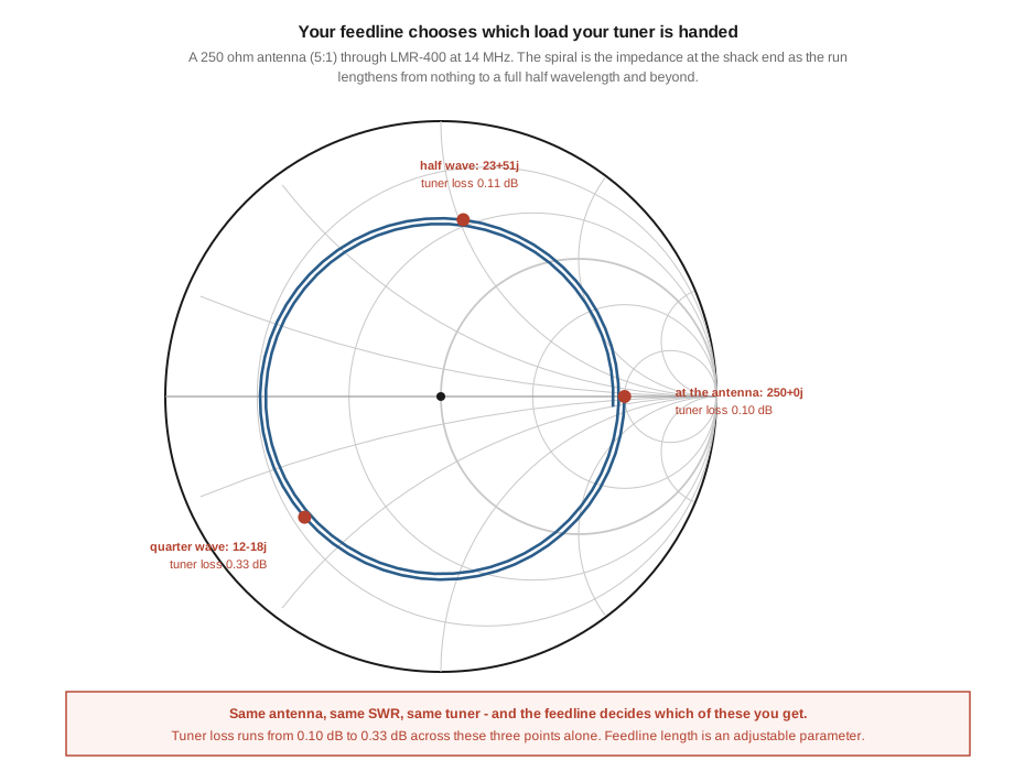
Take a fixed antenna — 250 Ω resistive, a 5:1 mismatch — and lengthen the coax between it and the tuner. The impedance at the shack end traces the spiral in the figure, running once around the chart every half wavelength and creeping inward as loss attenuates the reflection. Three lengths, three quite different loads:

Table 5 — Take a fixed antenna — 250 Ω resistive, a 5:1 mismatch — and lengthen the coax between it and the tuner. The impedance at the shack end traces the spiral in the figure, running once around the chart every half wavelength and creeping inward as loss attenuates the reflection. Three lengths, three quite different loads

feedline	load at the tuner	SWR	tuner loss
at the antenna	250 + j0	5.00:1	0.10 dB
a quarter wave	12 − j18	4.90:1	0.33 dB
a half wave	23 + j51	4.67:1	0.11 dB

Same antenna, same tuner, essentially the same SWR — and the tuner’s loss varies by a factor of more than three depending on how much cable is between them. Feedline length is a parameter that moves you around Vol 3’s loss curve without touching the antenna.

This is the practical lever that volume identified and could not act on. If your tuner runs hot on one band, adding or removing a few feet of coax moves the load to a different point on the spiral, and on the low-resistance side of the chart a few feet can be worth several tenths of a decibel. It is also why a station that works beautifully on five bands and fights on the sixth is usually suffering from a feedline length rather than an antenna problem — and why “try a different length of coax”, which sounds like superstition, is sound engineering advice.

⚠ The obvious caution: changing the length moves every band at once, and a length that helps on 40 m may hurt on 20 m. This is an optimisation across bands, not a fix, and it is best done with the measurement from §2 and a transmission-line calculator rather than by cutting cable and listening.

4.6.1 When hand-matching still earns its keep

An autotuner costs less than a good roller inductor and finds a match in under a second. Four cases still favour doing it yourself.

High power. Autotuners switch with relays and fixed component banks; the voltage and current inside a matching network at a kilowatt are what Vol 2 computed, and they are unkind to relay contacts. Manual tuners with air-spaced variables remain the high-power answer.

Loads outside the search space. An autotuner has a finite bank of L and C values, and it will report failure on a load a continuously-variable network handles easily. That is a component-value limit, exactly as Vol 2 §6 described for the L-network.

Diagnosis. When a tuner will not match, the Smith chart tells you why — the load is off the reachable region in a specific direction, and the fix follows from which direction. That is a diagnosis an autotuner’s blinking light cannot give you.

Knowing which solution you got. This is the strongest case and it runs through the whole dive. An autotuner searches until the SWR bridge is satisfied and then stops. It has no way to prefer the low-Q route over the high-Q one, or the all-capacitor solution over the one that puts the coil in circuit, because the quantity it optimises is the one quantity that cannot distinguish them. A network set by hand, from a measured load, on a chart, can be the good solution rather than a solution — and on the numbers in §5 that is worth more than the time it costs.

4.7 Where this volume hands off

The load is measurable in twenty minutes at the plane the tuner will meet, and it is the number the previous three volumes kept needing. Read on a Smith chart — which this chapter previously described wrongly in three of five particulars, including a sentence that contradicted itself — an L-network is two moves: one to land on the r = 1 or g = 1 circle, one to slide along it to the centre. There are generally four ways to do it, they differ in Q by a factor of two and in loss by a factor of eight, and the best of them is usually the one that leaves the inductor out of circuit. And the length of coax between antenna and tuner is a real adjustment that moves you around the loss curve, worth a factor of three on the numbers here.

The chapter’s matching procedure had the two moves in the wrong order for both configurations — the same inversion as its schematics, stated two paragraphs after the correct rule. That is the second independent appearance of one misunderstanding, and it is why nothing in this dive has been taken on trust.

From here:

• Vol 5 — DIY build and buys builds the 80–10 m L-network Vol 2 derived, at 200 W, and verifies it against a measured load using §2’s method. It is also where the commercial survey lives — and where §5’s “leave the coil out” finding becomes a question about what topology to buy, since most of the market cannot offer the choice.
• Vol 1 and Vol 3 are the two this volume answers. Vol 1 asked what the tuner reaches; Vol 3 showed that the load decides the cost; §2 here is how you find out what it is.

Two things are owed. No measurement in this volume is mine — the method in §2 is standard and the numbers throughout are computed, but a bench session sweeping a real antenna at a real shack-end plane, and then setting a real tuner from the result, is the demonstration this volume wants and does not have. And §5’s all-capacitor finding deserves a bench check before it is leaned on hard: the capacitor-Q figure used here is a conservative estimate rather than a measurement of any specific component, and while the direction of the result is not in doubt, the factor of eight is only as good as that estimate.

4.8 Resources

• NanoVNA, Vol 3 — calibration and the three-term error model, which is the part of §2 that decides whether your measurement means anything.
• NanoVNA, Vol 4 — S11, the Smith chart display, and time-domain reflectometry. The companion to §3 from the instrument’s side.
• Philip Smith, Electronic Applications of the Smith Chart — the chart from its inventor. Still the clearest account of why the transformation is the right one.
• David Pozar, Microwave Engineering, Ch. 2 and Ch. 5 — the chart’s construction and the L-network’s two solutions, derived rather than asserted.
• S. E. Hunt, G3TXQ, What tuners do — the worked doublet whose network §5 reproduces, and the source of the impedances used throughout this dive.
• N6BV, TLW (ships with the ARRL Antenna Book) — the transmission-line calculator for §6’s feedline-length question, carrying a complex characteristic impedance as Vol 3 requires.
• Antenna tuners, Vol 3 — why the load is the variable that decides, and the loss curve §6’s spiral walks along.
• BALUNs and UNUNs, Vol 1 — common-mode current, the measurement artefact §2 warns about and the reason it is worth fixing rather than working around.
• Antenna theory and practice — reflection coefficient, SWR and impedance from first principles, if §3’s vocabulary needs shoring up.