Four Ports, and What the Phase Buys

---

3.1 About this volume

Vol 1 established that a three-port network cannot be matched, lossless and reciprocal at the same time, and Vol 2 showed how the Wilkinson evades the consequence by carrying a resistor that draws no current. There is a second escape, and it is more radical: stop building a three-port.

The theorem is specific to three ports. A four-port network can be simultaneously lossless, reciprocal and matched at every port, with perfect isolation between two chosen pairs, and no resistor anywhere. The branch-line hybrid, the rat-race ring and the coupled-line coupler are all such networks. They pay for it in two ways — a fourth port that must exist and must be terminated, and a bandwidth generally narrower than a Wilkinson’s — and they are rewarded with something a three-port cannot offer at all: the phase relationship between the outputs becomes a design parameter. That is what the whole family is for.

The seed chapter’s treatment of these devices contains the dive’s two most consequential drawing-level errors, and both were found by computing the network rather than reading the description.

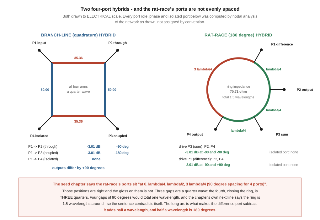
The first is that its rat-race geometry contradicts itself in consecutive lines. It states the ring is 1.5 wavelengths in circumference and then that the four ports are at “90 degree spacing”. Four gaps of 90° total one wavelength, not one and a half. §5 shows the correct arrangement — three gaps of a quarter wave and a fourth of three quarters — and, more usefully, why that long arc is the entire mechanism of the device.

The second is that its bandwidth ranking of the two hybrids is inverted. The chapter gives the rat-race “~15 %” and calls it “narrower than Wilkinson; narrower still than quadrature”. Computed against a stated threshold, the rat-race is 22.6 % and the branch-line is 10.4 % — the rat-race is more than twice as wide as the quadrature hybrid it is said to be narrower than. This is the fourth inverted claim this program has found in a seed chapter, after the receive-loop dive’s K9AY direction, the transmitting-loop dive’s radiation pattern and the end-fed dive’s odd harmonics.

A third result is not a correction but is the most practically useful thing here: §4 finds that a branch-line hybrid’s amplitude balance degrades far faster than its phase relationship, which is the reverse of what the chapter’s own myth-list implies and of what most engineers assume.

3.2 The fourth port changes what is possible

The three-port argument of Vol 1 §2 turned on counting: with the diagonal zeroed and the matrix symmetric, unitarity forces two of the three couplings to vanish. Run the same argument on a four-port and it does not close. There is enough freedom in a 4 × 4 unitary symmetric matrix with a zero diagonal to satisfy every constraint at once, and the general solution is the directional coupler condition — port 1 couples to ports 2 and 3, and not at all to port 4; port 2 couples to ports 1 and 4, and not at all to port 3. The ports pair off into two isolated pairs.

That structure has a consequence worth stating before any specific device. In a lossless four-port with this pairing, the two outputs are necessarily in phase quadrature relative to one another in a fixed way determined by the topology, because unitarity constrains the phases as tightly as it constrains the magnitudes. The 90° of a branch-line and the 180° of a rat-race are not design choices layered on top of the splitting function; they fall out of the same requirement that makes the device work at all. This is why there is no such thing as a lossless, matched, isolated four-port with two in-phase outputs and nothing else — the phase has to go somewhere.

The fourth port is not optional and it is not free. In a branch-line used as a splitter it is the isolated port, and it must be terminated in a good 50 Ω load, because anything reflected from it re-enters the network and destroys the isolation the device was chosen for. In a rat-race used as a combiner it is the difference port, and terminating it is what absorbs the mismatch between the two inputs — playing exactly the role the isolation resistor plays in a Wilkinson, and for exactly the same reason. Vol 1 §6’s table of where combined power goes applies here without modification; only the component that absorbs it has changed from a chip resistor to a coaxial termination.

3.3 The branch-line hybrid, computed

The branch-line is a square of four quarter-wave transmission lines. Two opposite arms — the ones carrying the through path — have characteristic impedance Z₀/√2 = 35.36 Ω; the other two have Z₀ = 50 Ω. The seed’s §5.1 diagram labels the arms 35.4 Ω and 50 Ω, and that labelling is correct and should not be re-opened.

Analysing the network as drawn — assembling the nodal admittance matrix from the four arms and converting to S-parameters — gives, at the design frequency, driving port 1:

Table 1 — Analysing the network as drawn — assembling the nodal admittance matrix from the four arms and converting to S-parameters — gives, at the design frequency, driving port 1

path	magnitude	phase
P1 → P2 (through)	−3.01 dB	−90°
P1 → P3 (coupled)	−3.01 dB	−180°
P1 → P4 (isolated)	none	—
P1 → P1 (reflection)	none	—

Perfectly matched, perfectly isolated, an exact 3.01 dB split, and 90° between the two outputs, which is the device’s purpose.

The seed describes the outputs as “Output 1 (0°)” and “Output 2 (−90°)”. The difference is right, and the difference is the only thing that matters in every application, so this is a small correction rather than a substantive one. But neither output is at 0°: they are at −90° and −180°, because both paths traverse at least one quarter-wave arm and the coupled path traverses two. An absolute phase of zero would require a path of zero electrical length, and there isn’t one. The distinction matters only when a hybrid is embedded in a larger phased structure where absolute path length is being budgeted — which is exactly the case in the antenna-feed application of §7.

The chapter also gives the isolation as “25–30 dB”. As with the Wilkinson in Vol 2, the ideal figure at the design frequency is infinite — the computation above returns the solver’s numerical floor, not a finite value — and 25–30 dB is what a real part achieves once construction tolerance, connector discontinuities and the termination on port 4 are accounted for. The quoted range is a realistic manufactured figure and is retained as such; what is wrong is only the implication that it is a property of the topology.

3.4 The amplitude fails before the phase does

The chapter’s myth list contains this entry: “All quadrature hybrids are 90° phase — true at center frequency, false at band edges. Phase response is frequency-dependent; the 90° spec is at the design center, with ±10° variation across the band typical.”

Computing the phase difference across frequency confirms the figure. At f/f₀ = 0.9 the outputs differ by 88.78°, an error of 1.2°; at 0.8 they differ by 81.64°, an error of 8.4°. Over a ±20 % band the phase error stays inside about ±10°, exactly as the chapter says. Confirmed, not corrected.

What the same sweep shows, and the chapter does not, is that the phase is the robust half of the specification:

Table 2 — What the same sweep shows, and the chapter does not, is that the phase is the robust half of the specification

f/f₀	phase difference	phase error	amplitude imbalance	isolation
0.80	81.64°	8.4°	1.835 dB	10.2 dB
0.90	88.78°	1.2°	0.577 dB	14.9 dB
1.00	90.00°	0	0 dB	exact
1.10	91.22°	1.2°	0.577 dB	14.9 dB
1.20	98.36°	8.4°	1.835 dB	10.2 dB

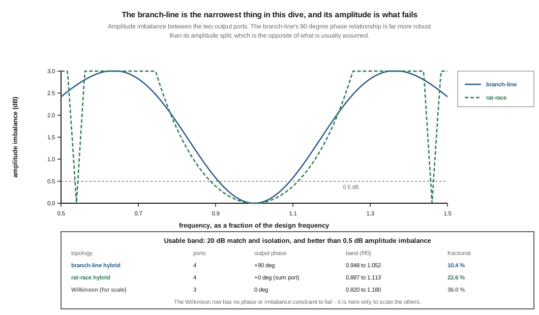
At f/f₀ = 0.9 the phase is within 1.2° of perfect while the two outputs already differ in amplitude by 0.577 dB — a 14 % power difference. By 0.8 the phase error is still a tolerable 8.4° while the amplitude imbalance has reached 1.8 dB, which is a 50 % power difference and unusable for most of the applications in §7.

The branch-line hybrid is an accurate phase-shifter with a mediocre power split, not the other way round. That has a direct design consequence: in a balanced amplifier, where the hybrid’s job is to drive two devices equally and in quadrature, the specification that runs out first is gain balance between the two devices, not phase tracking. And it explains why the usable band computed on a combined criterion — better than 20 dB return loss and isolation, and better than 0.5 dB amplitude imbalance — is only 10.4 %, far narrower than the phase specification alone would suggest.

For completeness, and because the seed gives the branch-line “~20 %” with no threshold attached in the same way Vol 2 §5 found for the Wilkinson: relaxing the criterion to 15 dB and 1.0 dB of imbalance gives 18.4 %, and tightening it to 25 dB and 0.25 dB gives 5.8 %. The chapter’s 20 % is the loose figure. This is the fourth appearance of the missing-threshold defect in this hub.

3.5 The rat-race, and a ring that cannot be what it says it is

The rat-race is a closed ring of transmission line with four ports tapped onto it. The seed gets the circumference right — 1.5 wavelengths — and then says of the port positions: “at 0, λ/4, λ/2, 3λ/4 (90° spacing for 4 ports)”.

Those four positions are correct. The gloss on them is not, and it is arithmetically impossible. Four ports at positions 0, λ/4, λ/2 and 3λ/4 divide the ring into gaps of λ/4, λ/4, λ/4 and — closing the ring from 3λ/4 back to 0 — 3λ/4. Three quarter-waves and one three-quarter-wave sum to 1.5 λ, which is the circumference the chapter itself states one line earlier. Four gaps of 90° would sum to one wavelength, contradicting it. The parenthesis and the circumference cannot both be true, and the circumference is the one that is right.

This is not a pedantic point about a diagram, because the long arc is the entire mechanism of the device. The lead figure draws both rings to electrical scale, which makes the asymmetry visible: a quarter wave is 60° of the drawing and the long arc is a full 180°.

The ring impedance is Z₀√2 = 70.71 Ω throughout — a figure the seed never states anywhere, which is a substantive omission in a chapter that a builder might work from.

Computing the network gives the port roles directly rather than by assumption. Driving the port opposite the long arc:

Table 3 — Computing the network gives the port roles directly rather than by assumption. Driving the port opposite the long arc

drive	outputs	phase	isolated
P3 (the sum port)	P2 and P4, both −3.01 dB	both at −90°, i.e. in phase	P1
P1 (the difference port)	P2 and P4, both −3.01 dB	−90° and +90°, i.e. 180° apart	P3

The mechanism is now readable. A signal entering the sum port reaches both outputs through a quarter wave, so they are in phase. A signal entering the difference port reaches one output through a quarter wave and the other through the long three-quarter-wave arc — a path difference of half a wavelength, which is 180°. The device subtracts because one of its arcs is half a wavelength longer than the other, and that half wavelength is precisely what the “90° spacing” gloss deletes.

The seed’s own §6.2 statement — “Phase: 180° between outputs in one configuration; 0° in another” — is therefore exactly right, and is confirmed here rather than corrected. The chapter knew what the device does. Its geometry note described a different device.

3.6 The ranking is the wrong way round

The seed gives the rat-race a bandwidth of “~15 %” and characterises it as “narrower than Wilkinson; narrower still than quadrature”. Computed on the same combined criterion for both — better than 20 dB return loss and isolation, and better than 0.5 dB amplitude imbalance between the outputs:

Table 4 — The seed gives the rat-race a bandwidth of "~15 %" and characterises it as "narrower than Wilkinson; narrower still than quadrature". Computed on the same combined criterion for both — better than 20 dB return loss and isolation, and better than 0.5 dB amplitude imbalance between the outputs

topology	ports	output phase	band (f/f₀)	fractional bandwidth
branch-line hybrid	4	+90°	0.948 to 1.052	10.4 %
rat-race hybrid	4	0° (at the sum port)	0.887 to 1.113	22.6 %
Wilkinson (for scale)	3	0°	0.820 to 1.180	36.0 %

The rat-race is more than twice as wide as the branch-line, not narrower than it. The chapter’s ordering of the two hybrids is inverted. Its placement of both below the Wilkinson is correct, and the Wilkinson row is included only to scale the other two — it has no phase or imbalance criterion that could fail, so its number is not measuring quite the same thing.

The mechanism behind the inversion is worth understanding rather than just recording. The branch-line’s four arms have two different characteristic impedances, and the impedance ratio between the arms is what sets both the split ratio and the match. Away from the design frequency those two functions detune at different rates and the split ratio drifts quickly — which is §4’s amplitude imbalance. The rat-race’s arms are all the same impedance, and its function depends on a path-length difference rather than an impedance ratio. A path-length difference of half a wavelength is wrong by the same fractional amount at any frequency, so the 180° relationship degrades gently and symmetrically, while the amplitude split, being set by identical arms, barely drifts at all.

The device whose behaviour rests on lengths is more tolerant than the device whose behaviour rests on impedance ratios. That generalises, and it is the reason the rat-race is the preferred choice whenever the application can use 0°/180° rather than quadrature.

3.7 What the phase actually buys

The seed lists the applications correctly and explains none of them, so this section supplies the mechanisms. Each is a case where the quadrature or antiphase relationship does work no in-phase splitter could do.

The balanced amplifier. Two nominally identical amplifiers are driven from a quadrature hybrid and their outputs recombined in a second quadrature hybrid. The reason is not power — two amplifiers give 3 dB whatever the phasing — but input match. Whatever each amplifier reflects from its input travels back into the hybrid, and the two reflections arrive at the input port having traversed different numbers of quarter-wave arms: they arrive 180° apart and cancel, while at the isolated port they arrive in phase and are absorbed in its termination. The result is that a balanced pair presents a good input match even when the individual devices do not, which is why the topology dominates broadband amplifier design where a device’s optimum noise match and optimum input match are at different impedances. The price is that the isolated port’s termination now absorbs the whole of the reflected power, so it must be rated accordingly.

Image-reject and single-sideband mixing. Two mixers driven 90° apart produce sum and difference products whose relative phases differ between the wanted sideband and the image. Recombining through a second quadrature network adds one coherently and cancels the other. The rejection achieved is set directly by how well the quadrature is maintained — and §4’s finding applies with force here, because in this application amplitude imbalance and phase error contribute jointly to the residual image. An imbalance of 0.577 dB alone, with perfect quadrature, limits image rejection to about 30 dB; that is the f/f₀ = 0.9 row of §4’s table, and it is why wideband image-reject mixers use amplitude-corrected hybrids rather than a bare branch-line.

Circular polarisation. Feeding two orthogonal linear antennas — crossed dipoles, or the two orthogonal feeds of a patch — with equal amplitudes 90° apart produces circular polarisation, and the sense is set by which feed leads. This is the application the satellite work depends on, and the satellite antennas and rotators dive covers the antenna side. The relevant fact from this volume is that axial ratio, the measure of how circular the polarisation really is, is set by the hybrid’s amplitude imbalance more than by its phase error. A 0.577 dB imbalance with perfect quadrature gives an axial ratio of about 0.58 dB; a 10° phase error with perfect amplitude gives about 0.76 dB. Both are good, but the amplitude term is the one that degrades first as the band is widened, for the reason §4 established.

Differential drive. The rat-race’s 180° port feeds balanced structures directly — a balanced mixer, a dipole, a push-pull stage — without a transformer. This is the one application in the list where the rat-race and a BALUN are genuine alternatives, and the trade is bandwidth against loss: the BALUNs dive covers ferrite transmission-line transformers that are decades wide, against the rat-race’s 22.6 %. Above about a gigahertz, where a wound transformer becomes difficult, the ring wins by default.

3.8 Coupled lines, and why 3 dB is hard

The third four-port structure is two transmission lines run close enough together to exchange energy. Its coupling is set by the even and odd mode impedances of the coupled pair:

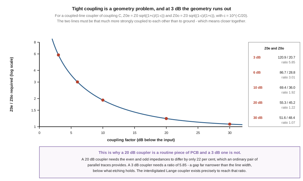
Z₀ₑ = Z₀√((1+c)/(1−c)) and Z₀ₒ = Z₀√((1−c)/(1+c)), where c = 10^(−C/20) for a coupling of C decibels

and the product Z₀ₑ Z₀ₒ = Z₀² always, which is the matching condition. Computing across the useful range:

Table 5 — and the product Z₀ₑ Z₀ₒ = Z₀² always, which is the matching condition. Computing across the useful range

coupling	Z₀ₑ	Z₀ₒ	ratio	through-path loss
3 dB	120.91 Ω	20.68 Ω	5.85	−3.02 dB
6 dB	86.74 Ω	28.82 Ω	3.01	−1.26 dB
10 dB	69.37 Ω	36.04 Ω	1.92	−0.46 dB
20 dB	55.28 Ω	45.23 Ω	1.22	−0.04 dB
30 dB	51.61 Ω	48.44 Ω	1.07	−0.004 dB

The ratio Z₀ₑ/Z₀ₒ is a direct measure of how strongly the two lines must couple to each other relative to how strongly each couples to ground — which, in a planar structure, is a statement about how narrow the gap between them must be relative to their width.

At 20 dB the ratio is 1.22. Two ordinary parallel traces separated by a comfortable gap achieve that, which is why a 20 dB PCB coupler is a routine object and why Vol 4’s measurement couplers are almost all in the 10 to 30 dB range.

At 3 dB the ratio is 5.85, and that requires a gap far narrower than the line width — in practice a few tens of micrometres on ordinary substrate, below what etching holds with any repeatability. This is precisely why the Lange coupler exists: by interdigitating the two lines into several interleaved fingers, it multiplies the coupled edge length without requiring an impossibly small gap, and reaches 3 dB in a manufacturable geometry. A reader who knows only that “couplers can be built on PCB” cannot predict that a 3 dB one needs a different structure entirely; a reader who has the ratio can.

The through-path column carries a second useful fact, and it answers one of the seed’s myths directly. Its list includes “Coupling and insertion loss are unrelated — false. For a fixed coupler topology, lower coupling (= more main-path power) means higher coupled-port loss.” The conclusion is right but the sentence is tangled. The clean statement is that in a lossless coupler the through path loses exactly the power the coupled port takes: 10·log₁₀(1 − c²). A 20 dB coupler removes 1 % of the signal, costing the main path 0.04 dB — genuinely negligible. A 3 dB coupler removes half, costing the main path 3.02 dB. The main-path loss of a directional coupler is not a defect of construction; it is the coupled power, and it is fully determined by the coupling factor.

3.9 Where this volume hands off

The four-port escape is real: a lossless, reciprocal, matched, isolated four-port exists, and the price is a fourth port that must be terminated and a band narrower than a Wilkinson’s. The branch-line gives 90° with arms at 35.36 and 50 Ω, is exactly matched and isolated at its design frequency, and holds its phase far better than its amplitude — 1.2° of phase error against 0.577 dB of imbalance at the 10 % band edge, which inverts the usual assumption about which specification to watch. The rat-race gives 0° at its sum port and 180° at its difference port from a 70.71 Ω ring, three of whose arcs are a quarter wave and the fourth three quarters — and that long arc is the whole mechanism, not a detail. It is 22.6 % wide against the branch-line’s 10.4 %, which is the opposite of the seed’s ranking, and the reason is that a path-length difference detunes more gracefully than an impedance ratio. Coupled lines cover the loose-coupling cases cheaply and run out of geometry at 3 dB.

One item is owed and is recorded rather than filled in. The seed’s §5.3 table of commercial quadrature hybrids lists a Mini-Circuits ZX10-2-12+ as a 90° hybrid. That designation could not be verified this pass — the manufacturer’s own store pages returned empty for this model — and there is a reason for suspicion, since Mini-Circuits’ quadrature parts are conventionally designated with a Q. That suspicion is recorded as a question, not asserted as a correction, because declaring a real product fictitious is a named failure mode in this program and has happened twice before. Vol 5 carries it into the commercial survey.

From here:

• Vol 4 — Sampling instead of splitting takes the coupled-line structure of §8 and puts it to the use it was invented for: measuring. The governing specification turns out not to be coupling but directivity, and Vol 4 turns a directivity figure into an error bar on an SWR reading. It also settles what is inside a NanoVNA, where the seed chapter and this hub’s own NanoVNA dive flatly disagree.
• Vol 5 — DIY build, measurement and buys builds, measures and surveys.

Every number in this volume comes from an idealised network of lossless lines and ideal terminations. Nothing here is a measurement.

3.10 Resources

• D. M. Pozar, Microwave Engineering, 4th ed., §7.5 (quadrature hybrid), §7.8 (180° hybrid), §7.6 (coupled line directional couplers) — the standard treatment of all three structures, including the even/odd analyses this volume computes numerically.
• J. Lange, Interdigitated Stripline Quadrature Hybrid, IEEE Trans. MTT, 1969 — the interdigitated coupler §8 names as the answer to the 3 dB geometry problem. Cited from its standard description in the literature rather than read first-hand.
• Passive splitters, Vol 2 — the Wilkinson, and the missing-threshold defect this volume finds for the fourth time.
• BALUNs and UNUNs, Vol 2 — the transformer alternative to the rat-race for differential drive, and the bandwidth comparison in §7.
• Satellite antennas and rotators — circular polarisation from the antenna side, the application of §7’s quadrature feed.
• NanoVNA, Vol 1 — the instrument, and the bridge-versus-coupler question Vol 4 settles.