Flooding the Sky: Turnstile, Eggbeater and Quadrifilar Helix

---

2.1 About this volume

Vol 1 established three things this volume spends: that circular polarization is mandatory at VHF and UHF because the ionosphere rotates a linear wave by hundreds of degrees; that a CP antenna’s axial ratio is a property of a direction rather than of the antenna, and is at its worst off boresight; and that a lossless antenna covering the whole upper hemisphere cannot exceed 3.01 dBi, however it is built.

Those three facts define a class of antenna, and this volume is about it: fixed, circularly polarized, low gain by design, pointed at the zenith once and never touched again. A turnstile, an eggbeater, a quadrifilar helix. No rotator, no controller, no zenith keyhole, no aiming, and — this is the part that decides it for most stations — nothing that can fail while the operator is asleep.

Three things in this volume differ from the seed chapter, and two of them are corrections to arithmetic that the chapter itself supplies the inputs for.

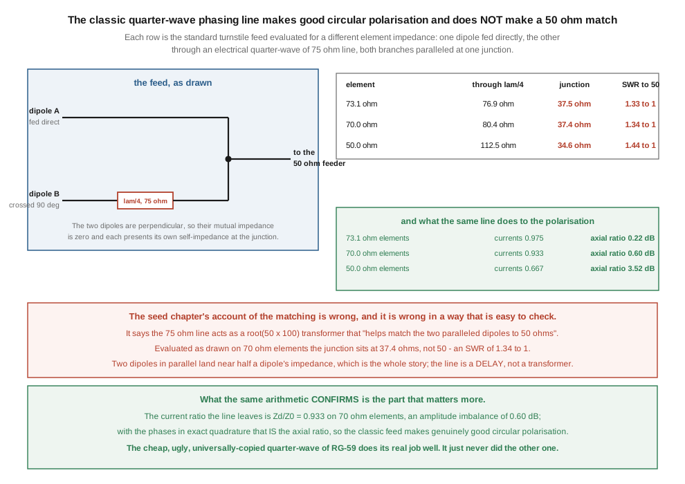
The turnstile’s phasing line does not do what the chapter says it does, and it does something better. §3 evaluates the canonical quarter-wave of 75 Ω line as drawn. The chapter says it acts as a √(50 · 100) transformer that helps match the paralleled dipoles to 50 Ω. It does not: the junction lands at 37.4 Ω, an SWR of 1.34:1. What it does do is leave the two dipole currents in a ratio of 0.933, an amplitude imbalance of 0.60 dB, which with the phases in exact quadrature is the axial ratio. The cheap universal quarter-wave of RG-59 makes genuinely good circular polarization and was never a matching transformer.

The quadrifilar helix is described three times and comes out three different antennas. §6 works it. The dimension table gives an axial length of 0.250 λ, the figure caption says 0.42 λ, and the prose says a length-to-diameter ratio of 0.4, which on the chapter’s own diameter is 0.066 λ. The three differ by factors of 1.68 and 3.78. The table is the one that is right, and it can be shown to be right by a test none of the three statements mentions.

And the satellites the chapter builds these antennas for no longer exist. §8 is the hardest fact in this dive. NOAA-18, NOAA-19 and NOAA-15 were decommissioned in June and August 2025, and no satellite anywhere now transmits APT. This changes less about the antenna than it sounds and more about the chapter’s build procedure than is comfortable.

2.2 The first decision, and why it is usually made wrong

Every satellite ground station makes one architectural choice before it buys anything: track the bird with a gain antenna, or flood the sky with a fixed one. The choice is usually framed as a trade of performance against cost, and framed that way it is nearly always decided wrongly, because the two sides are not measured in the same units.

The honest framing comes out of Vol 1 §7’s bound. A fixed antenna covering the whole upper hemisphere has at most 3.01 dBi to spend. A tracked crossed Yagi has 9 to 13 dBic. The gap is 6 to 10 dB, and Vol 1 §8 puts that against a link budget where the difference between a horizon pass and an overhead one is 12 dB — so the tracked antenna buys somewhat less than the difference between a good pass and a bad one.

Against that, the fixed antenna’s advantages are not decibels at all:

It works on every pass, including the ones nobody is watching. A tracked array works the passes the operator is present for. A fixed antenna feeding a receiver that runs unattended collects everything that goes over, which for weather satellites is the entire point and for a beacon-monitoring or SatNOGS-style station is the whole architecture.

It has no acquisition problem. A tracked array is pointed by a prediction, and at the start of a pass the prediction is at its least reliable and the signal at its weakest. A fixed antenna’s gain at 5 degrees elevation is whatever it is, but it is there at the instant the bird clears the horizon.

It has nothing that wears out. No gearbox, no control cable, no feedback potentiometer drifting with temperature, no coax rotating through a loop ten thousand times a year.

It is immune to the keyhole entirely. Vol 5 computes the azimuth rate a near-overhead pass demands and finds it exceeds what a Yaesu G-5500DC can deliver above 84 degrees of maximum elevation. A fixed antenna does not care: the best passes are exactly the ones a rotator handles worst and a fixed antenna handles best.

The case for tracking is narrower than the folklore and is worth stating precisely, because Vol 3 is about it: a tracked array is for links that a 3 dBi antenna cannot close at all. A weak linear transponder worked on SSB, an L-band digital downlink with a hard demodulation threshold, an uplink that must deliver usable EIRP. For an FM bird with a strong beacon, or for 137 MHz weather work, the fixed antenna is not the compromise — it is the correct engineering answer, and the rotator is the compromise.

2.3 The turnstile, and its phasing line evaluated as drawn

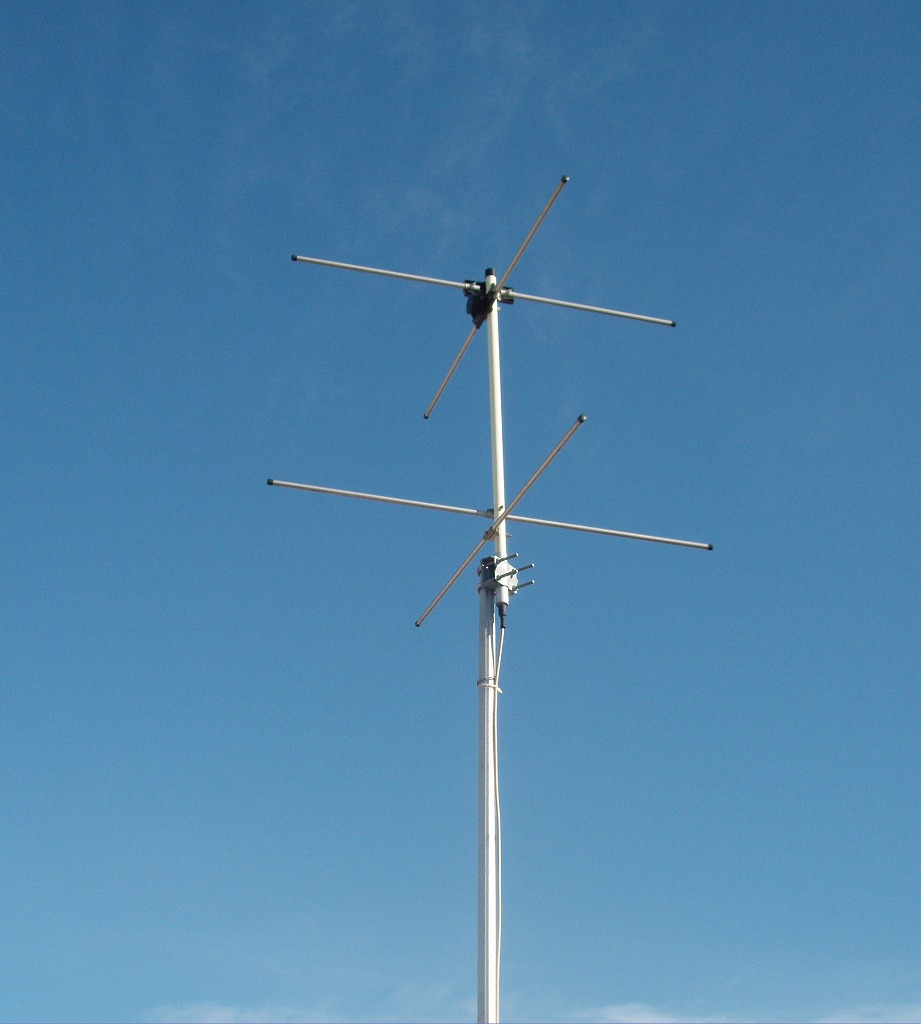
A turnstile is two half-wave dipoles crossed at 90 degrees in space and fed 90 degrees apart in time phase. Spatial quadrature plus temporal quadrature gives a field whose vector rotates at a constant rate: circular polarization, broadside to the plane of the dipoles, on both sides of it.

One structural fact makes the turnstile far simpler than it has any right to be, and the seed chapter states it without drawing the consequence. Two perpendicular co-located dipoles have zero mutual impedance. The fields of one are orthogonal to the current distribution of the other, so the coupling integral vanishes. Each dipole therefore presents its own self-impedance at the junction, unmodified by the presence of the other — which is why a turnstile can be designed by treating the two elements independently, and why the arithmetic in the lead figure is as simple as it is. In almost any other array of two driven elements this would not be true.

2.3.1 The phasing line, and what it actually does

The canonical feed is a quarter-wavelength of 75 Ω coax inserted in the path to one dipole, both branches then paralleled at a common junction and taken to a 50 Ω feeder. Reverse which dipole gets the delay and the sense flips between RHCP and LHCP.

The seed chapter’s account is this: “The classic phasing is a quarter-wavelength of 75 Ω line feeding the second dipole: an electrical 90° delay, with the 75 Ω impedance also acting as a √(50·100) transformer that helps match the two paralleled dipoles to 50 Ω.”

Evaluating that circuit as drawn takes two lines of transmission-line theory. The delayed branch presents the ordinary quarter-wave transform Z₀²/Z_d at the junction, in parallel with the direct dipole’s Z_d. And for a lossless quarter-wave with both branches sharing the junction voltage V, the load-end current of the delayed branch is |V|/Z₀ while the direct dipole’s is |V|/Z_d, so the current ratio between the two dipoles is Z_d / Z₀.

Table 1 — The phasing line, and what it actually does

element impedance	through the λ/4	at the junction	SWR to 50 Ω	current ratio	resulting axial ratio
73.1 Ω, the textbook half-wave	76.9 Ω	37.5 Ω	1.33:1	0.975	0.22 dB
70 Ω, trimmed to resonance	80.4 Ω	37.4 Ω	1.34:1	0.933	0.60 dB
50 Ω, a folded or shortened element	112.5 Ω	34.6 Ω	1.44:1	0.667	3.52 dB

🔴 The matching claim is wrong, and the arithmetic to see it is three lines long. The junction sits at 37.4 Ω, not 50 Ω. Nor could it have been otherwise: two dipoles in parallel land near half a dipole’s impedance, and the quarter-wave of 75 Ω moves the delayed one by 15 % rather than by the factor of two the √(50·100) story requires. The 100 Ω in that expression has no referent in the circuit. There is nothing in a turnstile that presents 100 Ω.

⚠ The practical consequence is small, which is why nobody has noticed. 1.34:1 is a perfectly acceptable SWR, and the antenna works. But an operator who believes the matching story will interpret a measured 1.3:1 as evidence that something is slightly wrong, and will chase it. The correct expectation is that a bare turnstile fed this way reads about 1.3:1 and that this is the design working, not failing. If a 50 Ω presentation is wanted, it comes from a quarter-wave transformer of about 43 Ω after the junction, or from accepting the 1.3:1.

⭐ What the same three lines confirm is the claim worth having. With the phases in exact quadrature, an amplitude imbalance of r between the two components produces an ellipse whose axial ratio is exactly r. So the current ratio column is the axial-ratio column. On 70 Ω elements the classic feed delivers 0.60 dB axial ratio on boresight, and on textbook 73.1 Ω elements 0.22 dB. Reading those against Vol 1 §5’s table: a matching-sense pair at 0.60 dB axial ratio loses about a hundredth of a decibel. The cheap, ugly, universally-copied quarter-wave of RG-59 does its real job extremely well.

🔴 And the third row is a design warning the seed chapter does not give. Feed the same network with 50 Ω elements — a folded dipole with a 4:1, or a shortened element brought down to 50 Ω — and the current ratio falls to 0.667, an axial ratio of 3.52 dB. That is outside what anyone would call good circular polarization, on boresight, before the pattern has degraded it any further. The quarter-wave phasing line only works well when the element impedance is close to the line impedance, and the reason the classic design uses 75 Ω line is that a half-wave dipole is close to 75 Ω, not because 75 Ω is a convenient transformer. Substituting 50 Ω coax for the phasing line, which is a common shortcut because it is what is in the junk box, makes the imbalance worse in the other direction.

The premium answer sidesteps all of it: a 90-degree quadrature hybrid coupler gives equal amplitudes and an accurate 90 degrees across a real bandwidth, and its fourth port makes the sense switchable with a relay. Vol 3 covers that, because it matters more on a tracked array where the sense can be chosen per bird.

2.4 The reflector, and the 3 dB it is actually buying

A bare turnstile radiates circularly on both sides of the plane of its dipoles — upward, which is wanted, and downward, which is not. Placing a reflecting screen or a set of reflector rods below the dipoles suppresses the downward lobe and pushes the pattern into the upper hemisphere.

The gain that buys is not a mystery and it is not a matter of opinion: it is Vol 1 §7’s bound read forwards. Halving the solid angle an antenna radiates into doubles its directivity, so a perfect reflector is worth up to 3.01 dB and no more. A real one is worth somewhat less, and the shortfall goes into the pattern distortion and the residual back lobe.

⚠ On the spacing, this dive declines to correct the seed and says why. The seed chapter specifies a reflecting screen “about 0.3 λ below” the dipoles. General reference sources give a quarter wavelength. Both figures are in wide circulation, and they are not describing quite the same thing: the spacing trades the depth of the null below against the shape of the pattern at low elevation, and a design that wants gain near the horizon uses a different spacing from one that wants maximum gain at the zenith. No source was found that settles which figure the seed intended, and the difference is under 20 % of a quantity whose optimum is broad. It is recorded here as a range rather than resolved, and §10’s build uses the seed’s 0.3 λ so that a reader comparing the two documents is not sent off on a different antenna.

⭐ The interesting consequence is one the seed chapter does not draw. A turnstile with a reflector below it has its maximum gain at the zenith and falls away toward the horizon, which is the wrong shape for a LEO pass. Vol 1 §8’s budget says the bird needs the most help at low elevation — longest slant range, worst multipath — and the reflector puts the gain where the link is already easiest. That is the specific defect §5 and §7’s antennas exist to address, and it is why a turnstile-with-reflector is a good weather antenna and an indifferent amateur-satellite one.

2.5 The eggbeater, and the horizon problem it exists to solve

An eggbeater replaces the turnstile’s straight dipoles with two crossed full-wave loops, again fed in quadrature, usually over a reflector or with a pair of reflector loops beneath. The loops give a pattern that is fatter at low elevation than a flat turnstile’s, so the antenna holds useful gain and useful circularity closer to the horizon.

That is the whole of the design intent, and stated against §4 it is a specific fix for a specific defect: the turnstile puts its gain at the zenith, the pass needs gain at the horizon, and the eggbeater moves some of the former to the latter. It does not violate Vol 1 §7’s bound — it is redistributing 3 dBi’s worth of coverage, not creating gain — and the price is paid overhead, where the link had margin to spare.

For FM birds worked with a fixed antenna, that redistribution is close to the ideal shape, and it is why the eggbeater has been the standard no-track amateur satellite antenna for thirty years.

⚠ The commercial position, however, could not be established, and §11 records that rather than filling it in. The seed chapter names the M2 EB-144 and EB-432 as “the canonical commercial examples”. On 17 September 2026 M2 Antenna Systems’ own catalogue does not list an eggbeater antenna; the only reference to the word on M2’s site is a blog post titled “Testing M2 Eggbeater Baluns”. The antenna is thoroughly attested in the amateur literature and a great many are in service, so the honest reading is that it has probably been retired rather than that it never existed — and that is a different claim from either the seed’s or its opposite.

2.6 The quadrifilar helix, described three incompatible ways

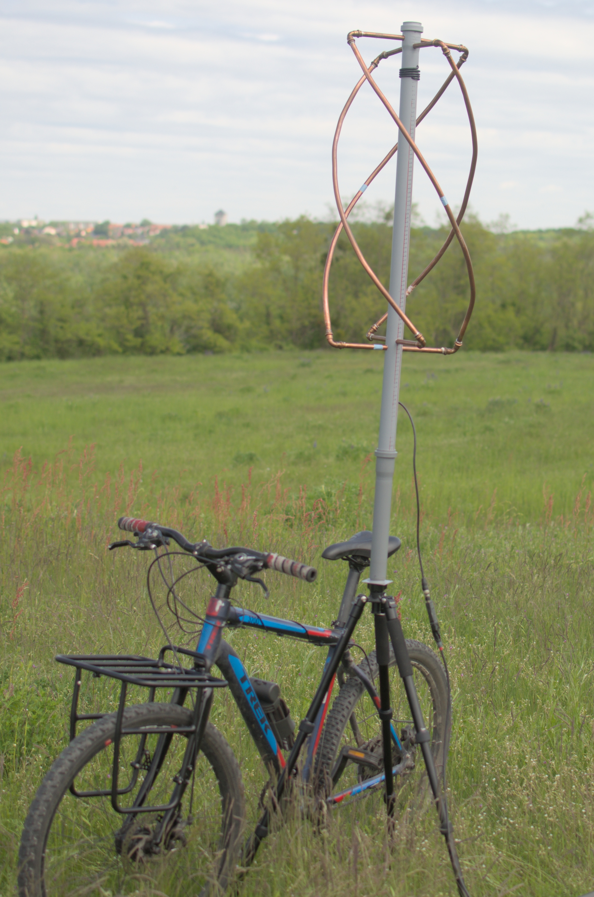
The quadrifilar helix is the antenna most associated with reliable unattended satellite reception, and it earns that by having the best pattern shape of anything in this volume: a broad, nearly hemispherical circularly-polarized lobe that stays useful most of the way down to the horizon, with no external phasing network at all.

The mechanism is the elegant part. Two bifilar helical loops are mounted orthogonally, and one is made slightly larger than resonance and the other slightly smaller. The larger loop is inductive and its current lags; the smaller is capacitive and its current leads. Sized correctly, each is offset by 45 degrees in the appropriate direction, and the two are therefore 90 degrees apart — the quadrature is produced by the geometry, and there is no phasing line to get wrong. Everything §3 had to say about the turnstile’s feed simply does not arise.

The price is mechanical. The geometry is fiddly to build accurately, and the dimensions are unforgiving, which makes it important that a builder is given the right ones.

2.6.1 Three statements, three antennas

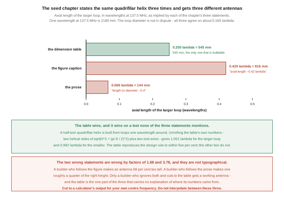
The seed chapter specifies its quadrifilar helix three times, in three places, and the three do not agree.

Its dimension table gives the larger loop a diameter of 360 mm and an axial length of 545 mm at a design frequency of 137.5 MHz. One wavelength there is 2,180 mm, so that is a diameter of 0.165 λ and an axial length of 0.250 λ, with a height-to-diameter ratio of 1.51.

Its figure annotates the same antenna with “Axial length H ≈ 0.42 λ”, which is 916 mm — 1.68 times the table.

Its prose instructs the reader to feed a calculator with “turns = 0.5, length-to-diameter ~0.4”. On the chapter’s own 360 mm diameter that is an axial length of 144 mm, a quarter of the table’s figure and 3.78 times smaller.

These are not typographical slips. They are three different antennas, and a builder following any one of them will build something the other two would call wrong.

⭐ The table wins, and it wins on a test that none of the three statements mentions. A half-turn quadrifilar helix is built from loops that are approximately one wavelength around — that is the design rule the whole family rests on. Unrolling the table’s own numbers gives the loop perimeter directly: each helical side is the hypotenuse of the axial height and half the circumference, √(H² + (πD/2)²), and the loop is two of those plus two end wires.

Table 2 — Three statements, three antennas

loop	diameter	axial length	computed perimeter
larger	360 mm	545 mm	1.051 λ
smaller	340 mm	515 mm	0.992 λ

The table reproduces the one-wavelength rule to within 5 %, and it puts the larger loop above a wavelength and the smaller below it — which is precisely the inductive-and-capacitive offset the self-phasing mechanism requires. The table is internally consistent with the physics of the antenna in two independent ways, and neither of the other two statements is consistent with it at all. Nothing else in the chapter’s three statements carries that kind of corroboration, and it is the sort of check that settles the question without needing an external source.

⚠ The length-to-diameter figure deserves one word of defence, because it is the statement most likely to be a misreading rather than an error. The QFH design calculators in common use take a length-to-diameter parameter, and different calculators define it against different lengths — the axial height, the total conductor length, or the loop’s unrolled length. A “0.4” that is correct for one definition is badly wrong for another. The seed’s prose may have carried a correct number across a definition boundary. That does not make it safe to follow: whatever it meant, a reader who types 0.4 into the calculator the chapter names and cuts to the result will not get the chapter’s own table.

The practical instruction, which §9’s build gives, is to cut to a calculator’s output for one’s own centre frequency and not to interpolate between the chapter’s three statements.

2.7 Lindenblad and big wheel, and the idea worth keeping from them

Two less common fixed antennas round out the family, and one of them carries an idea that the rest of this volume needs.

The big wheel is three half-wave loops arranged in a plane, producing a horizontally polarized omnidirectional pattern. It is not circularly polarized and it is not really a satellite antenna; it appears in these discussions because it is omnidirectional and because horizontal-polarization VHF nets use it. Its relevance here is as a control: an antenna that is genuinely omnidirectional in azimuth and has a thin pattern in elevation, which is Vol 1 §7’s other case — the one that can honestly have gain and still be useless for satellites.

The Lindenblad is four dipoles tilted around a circle and fed with a progressive phase, producing a circularly polarized pattern whose gain peaks toward the horizon rather than the zenith. That is the idea worth keeping, and it is the logical end of §4’s observation. If the link is hardest at low elevation and easiest overhead, then the correct pattern for a fixed satellite antenna is not hemispherical at all — it is one that deliberately under-illuminates the zenith and spends the recovered coverage near the horizon, compensating the slant-range loss with antenna gain so that the received power is closer to constant across the pass.

Read against Vol 1 §8’s budget, the size of the prize is clear: the range term alone varies by 12.1 dB between a horizon pass and an overhead one at 550 km. An antenna that gave up 3 dB overhead to gain 3 dB at the horizon would flatten a quarter of that. That is a larger effect than most of the decisions operators agonise over, and it is available from pattern shaping alone, at no cost in hardware.

⚠ Neither the Lindenblad nor the eggbeater achieves the ideal version of this; both are partial. But it is the right way to think about choosing among them, and it is a better criterion than the gain figure on the box — which, per Vol 1 §7, is bounded at 3.01 dBi for anything in this class and therefore cannot discriminate between them anyway.

2.8 What is left transmitting on 137 MHz

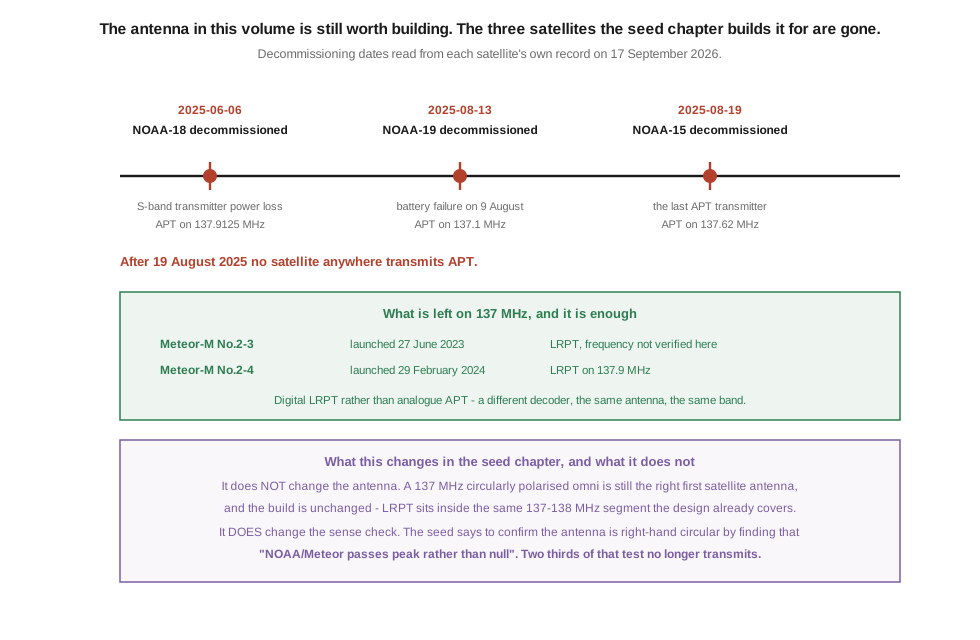
The seed chapter’s headline build is a 137 MHz antenna for “NOAA APT (137.1/137.9125/137.62 MHz) and Meteor-M LRPT”, and its recommended first purchase is a 137 MHz V-dipole described as “the default first weather antenna”. The three frequencies it gives were correct. The satellites are gone.

Table 3 — 8. What is left transmitting on 137 MHz

satellite	decommissioned	cause	APT frequency
NOAA-18	6 June 2025, 17:49 UTC	loss of power in S-band transmitter 4	137.9125 MHz
NOAA-19	13 August 2025, 16:55 UTC	battery failure on 9 August	137.100 MHz
NOAA-15	19 August 2025	the last APT transmitter in service	137.620 MHz

🔴 After 19 August 2025 no satellite anywhere transmits APT. NOAA-15, -18 and -19 each ran for between sixteen and twenty years against design lives of two, and the analogue picture-transmission service that had been continuously available since the 1960s ended within eleven weeks.

What remains in the band is digital: the Meteor-M series, of which No.2-3 (launched 27 June 2023) and No.2-4 (launched 29 February 2024) are operating. No.2-4’s low-rate picture transmission is on 137.9 MHz. ⚠ No.2-3’s LRPT frequency is widely quoted but was not verified for this dive and is not repeated here; a reader should take it from a current pass-prediction source rather than from this document.

2.8.1 What this changes, and what it does not

It does not change the antenna. This is worth saying first and plainly, because the temptation on discovering that a chapter’s targets are gone is to conclude that the chapter is obsolete. LRPT occupies the same 137–138 MHz segment, arrives from the same kind of polar orbit at the same elevations, and is right-hand circularly polarized like its predecessor. Every dimension in §9 and §10 is unchanged, and so is every argument in §2 through §7. A 137 MHz circularly polarized omni remains the correct first satellite antenna.

It does change what is on the other end, and therefore the receiver, the software and the expectations. APT was analogue FM that a cheap receiver could demodulate and that degraded gracefully into a noisy but readable image. LRPT is QPSK with a demodulation threshold: below it there is no picture at all rather than a poor one. A link that was marginal under APT produced a streaky image; the same link under LRPT produces nothing. That makes antenna quality matter more than it did, which is an argument for the quadrifilar helix over the V-dipole, and it makes the seed’s budget recommendation the weaker of the two rather than the sensible default.

🔴 And it breaks the chapter’s build-verification step, which is the operationally serious part. The seed’s QFH tuning procedure ends: “Confirm the sense is RHCP if that is your target by checking that NOAA/Meteor passes peak rather than null; if every pass is weak, you likely built LHCP.” Two thirds of that test no longer transmits, and the surviving third has a hard threshold, so “weak” and “absent” are no longer distinguishable by ear. §9 replaces the check.

⚠ One further consequence, recorded because it is a limitation of this dive rather than of the antenna. With APT gone, the easiest way to confirm that a home-built CP antenna has the sense its builder intended has gone with it. §9 gives two substitutes, neither as convenient as watching a NOAA pass peak.

2.9 DIY — a 137 MHz quadrifilar helix

The canonical unattended weather antenna, and an afternoon’s work. Centre the design on 137.5 MHz, which splits the band segment the surviving LRPT downlinks occupy.

2.9.1 Geometry

Use a published quadrifilar-helix calculator for a half-turn design and cut to its output for your own centre frequency. §6 established that the seed chapter’s three descriptions disagree, and that the one which survives its own consistency check is the dimension table:

Table 4 — Use a published quadrifilar-helix calculator for a half-turn design and cut to its output for your own centre frequency. §6 established that the seed chapter's three descriptions disagree, and that the one which survives its own consistency check is the dimension table

parameter	larger (lower) loop	smaller (upper) loop
loop diameter	360 mm (0.165 λ)	340 mm (0.156 λ)
axial length	545 mm (0.250 λ)	515 mm (0.236 λ)
twist	180° over the height	180° over the height
computed loop perimeter	1.051 λ	0.992 λ

⚠ Do not use the 0.42 λ from the seed’s figure or the 0.4 length-to-diameter from its prose. §6 shows both are inconsistent with the table and with the one-wavelength loop rule. The two rows of computed perimeter are the check to apply to any set of dimensions before cutting metal: the larger loop must come out a little above one wavelength around and the smaller a little below, because that asymmetry is the entire self-phasing mechanism. A set of dimensions that does not do that will not produce circular polarization whatever else is right about it.

The ±1 % sensitivity the seed warns about is real, and the antenna has no trim adjustment. It is a cut-once design.

2.9.2 Bill of materials

⚠ Prices are estimates, not quotations, and are given only to establish the order of magnitude. Nothing in this list was priced against a vendor for this dive.

Table 5 — Bill of materials

part	specification	note
support tube	40 mm PVC or fibreglass, ~800 mm	fibreglass if it will live in UV for years
spreaders	PVC tee fittings or a printed jig	the jig is what makes the geometry repeatable
loop conductor	RG-58 for the coaxial style, or 6–8 mm soft copper tube	copper tube holds its shape and is what the photograph above uses
downlead	LMR-240 or better, length to suit	it runs inside the support tube
common-mode choke	FT240-43 with ~8 turns, or a coiled-coax balun	not optional — see below
connector	BNC or SMA to suit the receiver
hardware	stainless screws, cable ties, sealant

2.9.3 Construction

Drill the support tube for the four conductor exits at the calculated top and bottom positions for each loop, offset 90 degrees around the tube. Form each conductor as a half turn from bottom to top. In the coaxial or “infinite balun” style the coax shield forms one half of the loops and the centre conductor crosses at the top feedpoint; the downlead runs inside the support tube and exits at the base.

The choke at the base is structural to the design, not a refinement. Common-mode current on the outside of the downlead radiates, and what it radiates is linearly polarized and arbitrarily phased with respect to the antenna. It therefore corrupts the axial ratio specifically — the one property the whole quadrifilar geometry exists to produce — and it does so without necessarily disturbing the SWR, so the fault is invisible to the only instrument most builders will point at it. Seal every penetration; this antenna lives outdoors for years.

2.9.4 Testing it, and the sense check the seed chapter can no longer make

Sweep it. A correct quadrifilar helix shows a broad return-loss dip below about 1.5:1 across 136–138 MHz with no sharp resonance; the antenna is inherently broadband, and a sharp resonance is itself a symptom. If the dip is off frequency the loops are mis-cut, and because there is no trim, the answer is to re-cut. See the NanoVNA dive for the sweep.

🔴 Do not use the seed chapter’s sense check. “Check that NOAA/Meteor passes peak rather than null” relied on satellites that no longer transmit, and on an analogue mode whose degradation was audible. Two substitutes, in order of confidence:

1. Check the geometry against the drawing before assembly. The sense is set by which way the conductors twist, viewed from the feed. This is deterministic and costs nothing, and it is the only check available before the antenna is finished. Photograph the partly-built antenna from directly above and compare with the calculator’s own diagram.
2. Compare against a known linear reference on a live pass. A correctly-sensed CP antenna and a linear dipole differ by Vol 1 §5’s exact 3.01 dB against a circularly polarized source, and the CP antenna’s signal will be steady where the linear one fades. The steadiness, not the level, is the diagnostic — and it is the diagnostic that survives the loss of APT, because it works on a digital downlink’s signal-strength indication as well as on an audible carrier. A wrong-sensed antenna will be down by Vol 1 §5’s figure, which at a realistic 3 dB axial ratio is 12.6 dB rather than the 20-plus the seed implies.

⚠ Neither substitute is as good as what was lost, and this dive does not pretend otherwise. The first proves only that the antenna matches its drawing; the second requires a second antenna and a pass. A measurement of axial ratio and sense on a rotating linear source at a known distance is the procedure that would settle it properly, and it is a bench task nobody in this dive has performed.

2.10 DIY — a 137 MHz turnstile with a reflector

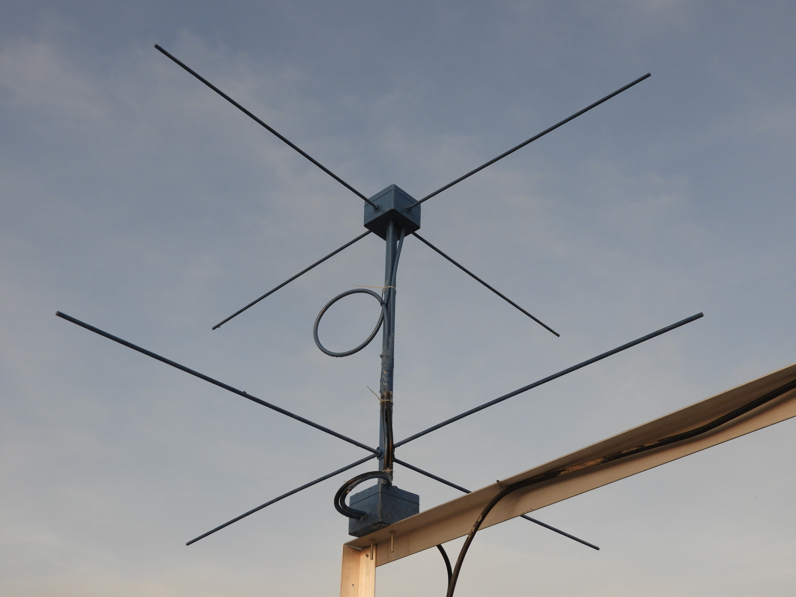
If the quadrifilar helix’s geometry is more than is wanted, the turnstile builds in an hour out of scrap and works.

Two half-wave dipoles for 137.5 MHz, each leg about 520 mm of aluminium rod or brazing rod, crossed at 90 degrees on a small plate or in a die-cast box. One dipole is fed directly; the other through an electrical quarter-wave of 75 Ω coax — for solid-polyethylene RG-59 with a velocity factor of 0.66 that is 0.25 × 2180 × 0.66 ≈ 360 mm of cable. Both branches join at one point and go to the feeder through a 1:1 choke balun. Four reflector rods, each slightly longer than the driven elements, sit about 0.3 λ (≈ 655 mm) below — subject to §4’s note on that spacing.

What to expect, from §3’s arithmetic rather than from optimism. The feedpoint will read about 1.3:1, not 1.0:1, and that is the design working correctly. The axial ratio on boresight will be around 0.6 dB if the elements are trimmed to resonance near 70 Ω. Use 75 Ω cable for the phasing line and not 50 Ω: §3’s third row shows what happens to the axial ratio when the element and line impedances diverge.

The choke is as non-optional here as it is on the quadrifilar helix, and for the same reason. The photograph above shows a builder who understood that: there is a coiled-coax choke at each feed, which is the detail that made it worth using as the illustration.

The turnstile is a touch less omnidirectional and a touch worse in axial ratio than a good quadrifilar helix, and per §4 it puts its gain at the zenith rather than where the pass needs it. For a first antenna built in an afternoon from scrap, those are the right compromises to accept.

2.11 Buys, dated

Everything in this section was checked on 17 September 2026. Where a figure could not be verified it is marked as unverified rather than filled in.

🔴 Most of the seed chapter’s fixed-antenna table could not be verified, and it is not repeated here. That table lists six products with price brackets. This dive was able to confirm the existence and current price of none of them, for a mixture of reasons — the manufacturers’ own sites were not reachable, the model designations did not resolve, or the product is not in the manufacturer’s current catalogue. Repeating unverifiable price brackets with a fresh date on them is the failure this program most wants to avoid, so the rows are withdrawn rather than refreshed.

Three specific findings are worth recording.

The M2 eggbeaters could not be found in M2’s catalogue. §5 gives the detail. The EB-144 and EB-432 are well attested in the amateur literature and many are in service; they are simply not in the current line as far as this check could establish. Treat them as a used-market entry.

The “RH-789” listed in the seed’s quadrifilar-helix row could not be matched to a quadrifilar helix product of any manufacturer, and is not repeated. ⚠ This is a withdrawal, not a claim that the product does not exist: the designation may belong to something else, or may be a transcription of a marketplace listing that has since gone.

MFJ Enterprises stopped manufacturing on 17 May 2024, taking Ameritron, Hy-Gain, Cushcraft, Mirage and Vectronics with it — a fact this project established in the antenna-tuners dive and which applies here because MFJ sold satellite and rotator accessories. ⚠ The nuance matters and is easy to get wrong in both directions. MFJ’s own web shop was live on 17 September 2026, states “We are still taking and shipping orders”, and lists both rotators and OSCAR antennas. That is remaining stock rather than production. An MFJ product found for sale is a real product that can be bought; it is not a product that will be made again, and it has no manufacturer behind its warranty in the ordinary sense.

2.11.1 What to look for instead of a price bracket

Since the product rows cannot be given honestly, the selection criteria can, and they follow from §§2–7 rather than from a catalogue:

Demand an axial-ratio figure, and demand the angle it applies at. Vol 1 §6: a CP antenna quoted without an axial ratio has said nothing about its polarization, and one quoted without an angle has given only its best case. This single test disqualifies most of what is sold as “satellite omni”.

Distrust any gain figure above about 3 dBi on an all-sky antenna. Vol 1 §7 makes this exact: 3.01 dBi is the hemispherical bound, and a higher honest number means a narrower cone. A listing claiming 8 or 9 dBi for an omnidirectional satellite antenna is describing something that is blind below roughly 48 degrees of elevation, whether or not it knows that.

Prefer a stated pattern to a stated gain. §4 and §7 show that for this class of antenna the shape is the whole specification and the peak number cannot distinguish a good one from a bad one.

For 137 MHz specifically, prefer a quadrifilar helix to a V-dipole now that the mode is digital. §8: LRPT has a threshold where APT had graceful degradation, so the margin a better antenna buys converts into pictures rather than into cleaner pictures.

A well-built commercial quadrifilar helix is worth buying for anyone who does not want to cut one, and §9’s build is worth doing for anyone who does. Both are correct answers; this dive cannot currently tell the reader what either costs.

2.12 Resources

• AMSAT (amsat.org) — the satellite status board and frequency lists; the list of active birds in this dive was read from it on 17 September 2026.
• The decommissioning dates in §8 were read from each satellite’s own record on 17 September 2026. The statement that no satellite now transmits APT is a direct quotation of the encyclopaedic record of the mode, not an inference from the three dates.
• John Coppens’ online quadrifilar-helix calculator — the community-standard half-turn QFH designer the seed chapter names. ⚠ The site was not reachable on 17 September 2026 and the calculator’s parameter definitions could not be checked; §6’s note on the length-to-diameter ambiguity is therefore unresolved rather than settled.
• SatDump — the current decoder for LRPT and the other digital weather downlinks, and the practical replacement for the APT software the seed chapter assumes.
• Vol 1 — the polarization loss, axial ratio and hemispherical gain bound this volume spends throughout.
• Vol 3 — the tracked antennas, and the quadrature hybrid that does §3’s job properly.
• Vol 5 — the keyhole arithmetic behind §2’s claim that the best passes are the ones a rotator handles worst.
• BALUNs and UNUNs — the common-mode choke that §9 and §10 both insist on, and why a choke fault is invisible to an SWR meter.
• NanoVNA — the sweep both builds are verified with.
• Satellite tracking — pass prediction, which is what tells the operator when to look at any of these antennas.