The Pattern

---

3.1 About this volume

Vol 1 separated the discone’s impedance bandwidth from its pattern bandwidth and left the second as a bound. This volume takes it up, and it is where this dive makes its largest correction.

The previous edition of this chapter states the discone’s elevation pattern, draws a diagram of it, builds a “good for scanning, bad for handhelds” trade-off on it, and then carries that trade-off into its best-case and worst-case sections. All of it rests on one description of where the antenna’s maximum response lies. That description is the reverse of the published account, and reversing it back inverts every conclusion drawn from it.

Two things need saying at the top about how this volume is argued, because the honest framing matters more here than anywhere else in the dive.

The published account is the authority; the computation is a model. Wikipedia’s discone article, sourced to the ARRL Antenna Book and Paul Lee’s handbook, says the antenna’s “sensitivity [is] highest in the direction of the horizon”. That sentence, not any calculation in this volume, is what contradicts the chapter. The elevation computations here exist to show the mechanism — why a radiator’s lobe sits on the horizon while it is short and leaves once it grows — and to establish at which end of the band each behaviour lives. A discone’s cone is fat and self-truncating and is not a thin vertical wire, so the exact angles below are illustrative. The direction of the effect, and which end of the band it belongs to, is what this volume claims.

The chapter’s claim is not invented, and saying so is part of the correction. A lifted main lobe at 25–35° is a real thing that really happens to these antennas. What the chapter does is state it as the discone pattern, unqualified, when it is the behaviour at the top of the range — and then give advice for the bottom of the range on the strength of it.

3.2 The claim, and the published account it contradicts

The chapter’s §7.1 is headed “The pattern is omnidirectional in azimuth but not peak-at-zenith” and reads:

A discone’s elevation pattern is the inverse of intuition — it doesn’t peak straight up. Instead, the pattern has:

• Peak elevation at ~25–35° above horizon (similar to a quarter-wave vertical)
• Null at zenith (no radiation straight up)
• Reduced gain near horizon (the cone’s apex points down at the horizon)
• Omnidirectional in azimuth (slight ripple, ±1 dB)

Item by item:

✅ “Null at zenith” is correct and is confirmed in §8. It follows from symmetry for any vertically polarised body of revolution and needs no modelling at all.

✅ “Omnidirectional in azimuth” is correct, though §6 shows the ripple figure is attached to the wrong structure.

🔴 “Peak elevation at ~25–35°” and “reduced gain near horizon” are the reverse of the published account. Wikipedia’s statement is unambiguous and is worth quoting at length because its second clause matters as much as its first:

The radiation pattern in the vertical plane is quite narrow, making its sensitivity highest in the direction of the horizon and rather less for signals coming from relatively close by.

That is the opposite claim in both halves. The published account puts the maximum at the horizon and the reduced response on high-angle signals arriving from nearby. The chapter puts a null at the horizon and the maximum at 25–35°.

🔴 And the parenthetical reason given is not a mechanism. “(the cone’s apex points down at the horizon)” — the cone’s apex points up; the cone hangs below the disc and flares downward, as every photograph in this dive shows. Even read charitably as “the cone’s surface slopes toward the horizon”, a conductor’s orientation is not what sets a radiation pattern; the current distribution is. There is no account here of why the response would be reduced at the horizon, which is usually the signature of a claim that was not derived.

⭐ One clause in the chapter’s own sentence points the right way and is overruled by the rest of it. It says the peak is “(similar to a quarter-wave vertical)”. A quarter-wave vertical over a ground plane has its maximum at the horizon — that is the defining property of the thing, the reason it is used for ground-wave and line-of-sight work, and the reason the fixed vertical monopoles dive treats it as the omnidirectional baseline. The chapter names the correct comparison antenna and then describes it incorrectly. This is the third time in this dive that the right answer has been present in the text beside the wrong one.

3.3 Where the maximum actually sits

The mechanism is the oldest result in vertical-antenna practice and it has a sharp threshold.

A vertical radiator of electrical height h over a ground plane has the elevation pattern

F(el) = | [ cos(k h sin el) − cos(k h) ] / cos el |

and the position of its maximum depends on h alone. Evaluating it:

Table 1 — and the position of its maximum depends on h alone. Evaluating it

frequency	radiator height	elevation of the maximum	horizon response, relative to the peak
1 × f_low	0.25 λ	0°	0.00 dB
1.5 × f_low	0.375 λ	0°	0.00 dB
2 × f_low	0.50 λ	0°	0.00 dB
2.5 × f_low	0.625 λ	0°	0.00 dB
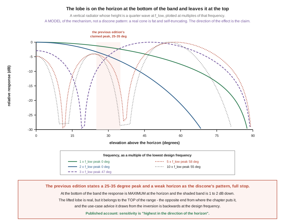
3 × f_low	0.75 λ	47.4°	−2.92 dB
5 × f_low	1.25 λ	57.8°	−4.88 dB
10 × f_low	2.50 λ	55.1°	−4.63 dB

Below 2.5 × f_low the maximum is exactly on the horizon. Not near it — on it. The response at 25–35° elevation over that whole span is 1 to 2 dB down from the maximum, which is the shaded band in the lead figure.

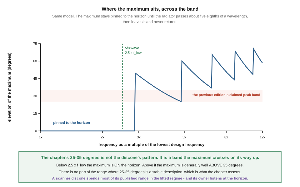
The threshold at 2.5 × f_low is not arbitrary: it is where a radiator whose height is a quarter wave at the bottom of the band reaches five eighths of a wavelength, which is the classical optimum for horizontal radiation. Wikipedia’s monopole article states it plainly — “Monopoles five-eights (5/8 = 0.625) of a wavelength long are also common, because at this length a monopole radiates a maximum amount of its power in horizontal directions” — and attributes the result to Stuart Ballantine’s 1924 work, which found “the amount of power radiated horizontally in ground waves reached a maximum at a mast height of 5/8 wavelength”.

⭐⭐ So the chapter’s 25–35° is not a place the maximum sits. It is a band the maximum crosses on its way up. Below 2.5 × f_low the maximum is at 0°; above it the maximum is generally well above 35°, sawtoothing between about 25° and 70° as successive lobes take over. There is no part of the frequency range over which “25–35°” is a stable description of anything, and that is what the chapter asserts it to be.

⚠ The usual objection, and why it does not rescue the claim. A vertical antenna over real, lossy ground does have its low-angle response attenuated by the ground reflection, and a pattern peak somewhere in the 20°–30° region is a thoroughly familiar sight in HF vertical modelling. If that is what the chapter’s number came from, the number has a real ancestor. But it would then be a property of the ground beneath the antenna, not of the discone, and it would be strongly dependent on height above ground, soil conductivity and frequency — none of which the chapter mentions. A scanner discone lives at VHF and UHF on a mast several wavelengths up, which is the regime in which ground effects are least like the HF case. Attributing a ground-reflection effect to the antenna’s own geometry is the error, whatever the number’s origin.

3.4 The lifted lobe is real, at the other end of the band

The correction is not that the discone’s lobe never lifts. It does, and Vol 1 §7 established the bound: a 1.70 m structure is 7.4 wavelengths tall at 1300 MHz and 17.0 wavelengths at 3000 MHz, and nothing that size keeps a single horizon-directed lobe. Wikipedia’s account agrees, in a sentence the chapter does not quote: “The elevation pattern might be distorted with grating lobes.”

So both descriptions are in the literature, and the whole of the correction is which end of the band each one belongs to:

Table 2 — So both descriptions are in the literature, and the whole of the correction is which end of the band each one belongs to

	bottom of the range	top of the range
electrical size	cone near λ/4	cone many λ
maximum	on the horizon	lifted, 25–70°, moving
the chapter says	lifted, 25–35°	lifted, 25–35°
published account	”sensitivity highest in the direction of the horizon"	"distorted with grating lobes”

⭐⭐ The chapter has taken the top-of-band behaviour, frozen it at one angle, and applied it across the whole range — including at the design frequency, where it is exactly wrong.

And the practical consequence is worse than a description error, because of where the published range puts the listener. A D130J is sold as 25–1300 MHz. Its cone reaches five eighths of a wavelength somewhere around 110 MHz. Above that — which is to say across the FM broadcast band, the airband, 2 m, the public-safety VHF and UHF allocations, 70 cm, and everything else a scanner owner actually listens to — the antenna is in the lifted regime, and the signals are at the horizon. The chapter’s error and the antenna’s real weakness point in opposite directions, and the real one is the one nobody is warned about.

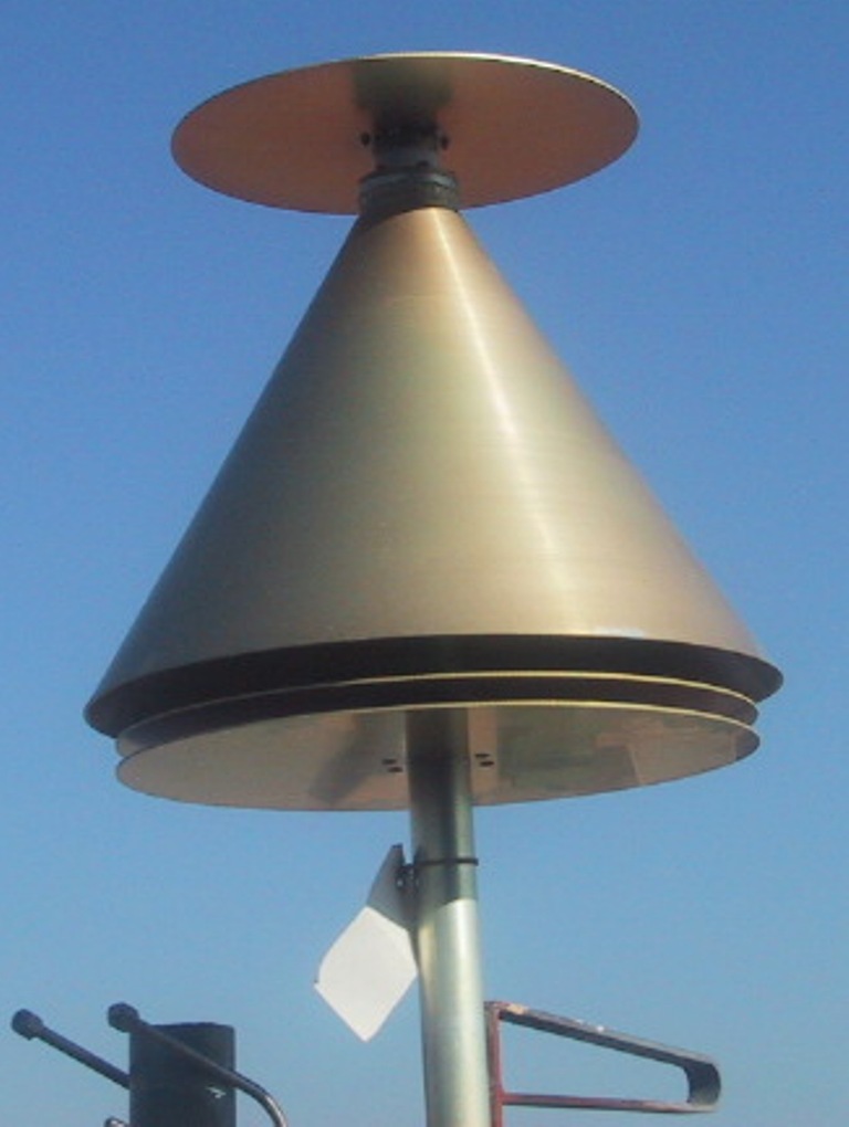
⚠ The photograph above is worth a note in this connection. It is a military-airband discone covering 225–400 MHz — a range of 1.8:1, not 50:1. A discone built for a narrow band can be proportioned so the whole band sits below the lifting threshold, and the extra skirt rings below the cone are the kind of feature that appears when a designer is optimising rather than stretching. The scanner discone’s pattern problem is a consequence of the 50:1 span being sold, not of the geometry.

3.5 The use-case advice, inverted

Because the chapter’s §7.2 reasons from the inverted pattern, its conclusions invert with it. The section is worth taking in full:

The discone’s elevation pattern is excellent for scanning (signals come in from elevated angles — repeaters on mountaintops, aircraft overhead, satellites passing) but suboptimal for horizon-line-of-sight receive of nearby vertically-polarized handhelds.

A 2 m handheld at horizon distance is essentially a horizon signal — the discone’s null at horizon means the handheld’s signal is reduced by 3–6 dB compared to a vertical or J-pole. For “monitor my local handheld friend,” a J-pole or vertical outperforms a discone.

🔴 There is no null at the horizon, and at the bottom of the band there is a maximum there. The specific claim that a handheld’s signal is reduced by 3–6 dB relative to a vertical is unsupported: at the frequencies in question a discone and a quarter-wave vertical both put their maximum at or near the horizon, and the discone’s published gain (§7) is within about a decibel of a vertical’s.

🔴 “Repeaters on mountaintops” is not an elevated-angle case, and this is the most consequential error in the section. A repeater on a mountaintop is typically many kilometres away. A site 600 m above the listener at 30 km distance subtends 1.1° of elevation. At 10 km it is 3.4°. Terrestrial VHF and UHF paths are horizon paths almost without exception — that is what makes them terrestrial — and the chapter has classified the single most common scanner use case as high-angle when it is the flattest geometry in the list.

⚠ Two of its examples are genuinely high-angle and should be kept. Aircraft directly overhead and satellites near the zenith really do arrive at steep elevations. But both run into §8’s zenith null rather than benefiting from a lifted lobe, and neither is helped by the pattern the chapter describes.

The corrected guidance, which mostly reverses the chapter’s:

• For terrestrial monitoring at the horizon — repeaters, public safety, marine, local handhelds, broadcast — a discone is at its best at the bottom of its range and progressively worse higher up as the lobe lifts. This is the opposite of the chapter’s advice and it is the main case.
• For aircraft and satellites at high elevation, a discone is mediocre at any frequency, not because of the lobe but because of the zenith null (§8). The chapter’s own worst-case section is right that a purpose-built antenna wins here.
• The chapter’s conclusion that a J-pole or vertical beats a discone for a local handheld happens to be defensible, but not for its reason. A single-band antenna beats a wideband one on any single band because it is resonant and the wideband one is not — which is the chapter’s own §15 myth entry, correctly argued there. ⭐ The right answer is in the chapter, three sections later, resting on the right mechanism.

3.6 Azimuth: the cone never ripples and the disc does

The chapter’s azimuth figures are:

A discone with 8 spokes has ~±0.5 dB azimuth ripple; with 16 spokes the ripple drops to ~±0.2 dB.

The structure of that claim — more spokes, less ripple, ripple attributable to the cone’s spoke count — is the same indexing error Vol 2 §5 found in the spoke-count rule, and it comes apart the same way.

Take N spokes equally spaced on a ring of radius a, in phase. The azimuthal array factor is

AF(φ) = Σₙ exp( j k a cos(φ − 2πn/N) )

whose azimuthal variation contains only harmonics of order N, 2N, 3N…, with amplitudes that stay negligible until ka approaches N. In plain terms: the pattern stays circular until the spacing between adjacent spokes approaches a wavelength.

Now apply it to the two rings a discone actually has.

The cone’s active ring scales with wavelength. Vol 2 §5 established that the radiating region sits near r = λ/4, so ka = 2π(1/4) sin θ — a constant, with no frequency in it. Evaluated at θ = 30°, ka = 0.785, and the ripple is:

Table 3 — The cone's active ring scales with wavelength. [Vol 2 §5](/discone-wideband/vol-2/) established that the radiating region sits near r = λ/4, so ka = 2π(1/4) sin θ — a constant, with no frequency in it. Evaluated at θ = 30°, ka = 0.785, and the ripple is

spokes	azimuth ripple, cone active ring
8	0.0000 dB
12	0.0000 dB
16	0.0000 dB

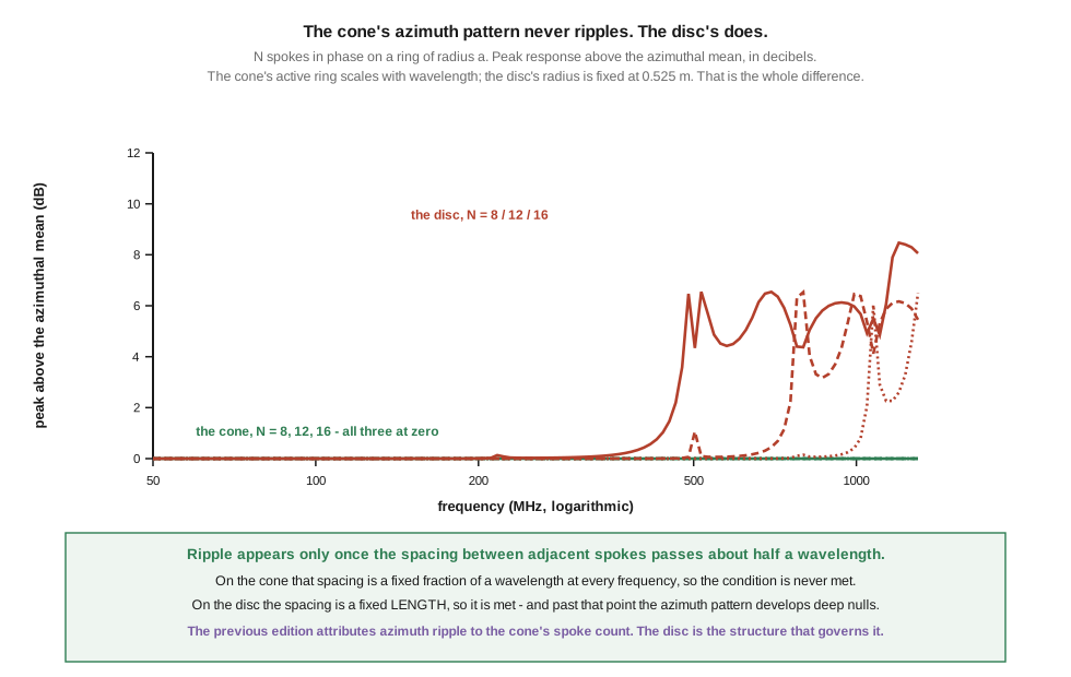
⭐⭐ Zero, at every frequency, for every spoke count above about six. Not small — numerically zero to four decimal places, because J₈(0.785) and its relatives are vanishing. The cone’s contribution to azimuth ripple is not a design trade-off; it does not exist.

The disc’s ring does not scale. Its radius is fixed at 0.7 × slant ÷ 2 — 0.525 m on a D130J-class antenna — so ka grows in proportion to frequency:

Table 4 — The disc's ring does not scale. Its radius is fixed at 0.7 × slant ÷ 2 — 0.525 m on a D130J-class antenna — so ka grows in proportion to frequency

frequency	disc spoke spacing	azimuth ripple, 12-spoke disc
50 MHz	0.046 λ	0.000 dB
144 MHz	0.132 λ	0.000 dB
450 MHz	0.413 λ	0.006 dB
800 MHz	0.734 λ	6.35 dB
1300 MHz	1.192 λ	5.45 dB

⭐⭐⭐ So the ripple is real, is far larger than the chapter’s ±0.5 dB where it appears at all, and belongs to the disc rather than to the cone. It switches on somewhere around half a wavelength of spoke spacing — between 450 and 800 MHz on this antenna — and above that the azimuth pattern develops deep nulls rather than gentle ripple. The non-monotonic behaviour between 800 and 1300 MHz is the Bessel oscillation and is characteristic.

⚠ This is a model and its limits should be stated. In-phase point sources on a ring are a crude stand-in for spokes carrying a decaying current distribution, and the absolute decibel figures should not be quoted as predictions. What the model establishes is structural and robust: which of the two rings can ripple and which cannot, and roughly where the threshold falls. That conclusion follows from one ring’s radius scaling with wavelength and the other’s not, which is a fact about the geometry rather than about the model.

⭐ And it resolves the asymmetry Vol 2 §5 asserted but could not quantify: the cone is frequency-independent in its discretisation and the disc is not. A builder adding spokes to the cone to clean up the high end is working on the wrong half of the antenna.

3.7 Gain, and the myth list

The chapter’s gain claims are its best-supported material and they check out.

“Discone has 6 dBi gain” — false. ~0 dBi to +2 dBi omnidirectional.

✅ Confirmed against a manufacturer’s own published figure. Diamond specifies the D130J at “Gain dBi: 2 (nominal)”, read on 17 September 2026. That sits at the top of the chapter’s stated range and comfortably refutes the 6 dBi claim the myth entry is aimed at. Wikipedia independently describes the discone as having “gain similar to a dipole”, which is 2.15 dBi. ⭐ Three independent sources agree with the chapter to within a few tenths of a decibel.

Two more of the chapter’s myth entries survive scrutiny and are recorded as confirmed so a later pass does not re-open them:

✅ “Discone is direction-finding” — false. Correct. §6 has just shown the azimuth pattern is circular to numerical precision through most of the range, which is the strongest possible statement of it. The nulls that appear at the top of the band are a disc artefact, not a bearing.

✅ “Discone gain is below a dipole” — true on a band-specific basis. Correct, and correctly reasoned: a 144 MHz dipole has 2.15 dBi at its design frequency against a wideband discone’s ~2 dBi across everything, and the single-band antenna wins on its band. This is the entry that should have carried §5’s handheld comparison.

⚠ One myth entry needs qualifying rather than correcting. The chapter writes: “‘The discone has a peak at the lowest frequency’ — false. The discone has roughly flat performance across its design band; it doesn’t peak at a single frequency.” The impedance is indeed flat across the band, which is Vol 1’s whole subject. But §3 and §4 have just shown that the antenna’s useful performance — response where the signals are — is best at the bottom of the range and degrades upward. So the entry is right about the match and wrong about the performance, and it is the exact place where the chapter’s conflation of the two bandwidths does its most direct damage to a reader.

3.8 Polarisation and the zenith null

Two properties are stated correctly by the chapter and are worth setting out properly, because they are what actually constrain the antenna’s high-angle use.

The discone is vertically polarised, and Wikipedia states it directly: “Omnidirectional, vertically polarized”. This follows from the geometry — a body of revolution about a vertical axis, fed against a horizontal disc, supports a current distribution with no net horizontal component in the azimuthal direction. It is the reason a discone is the right antenna for the vertically polarised services that dominate VHF and UHF monitoring, and the wrong one for horizontally polarised amateur SSB work on 2 m and 6 m, where the polarisation mismatch alone costs something like 20 dB.

The zenith null is genuine and is a hard consequence of symmetry. The chapter’s “Null at zenith (no radiation straight up)” is correct. Any vertically polarised radiator that is rotationally symmetric about the vertical axis must have zero response along that axis: the field there would have to point in some horizontal direction, and no direction is distinguished, so it must be zero. This is not an artefact of any model and no amount of design changes it.

⭐ That null is what really governs the satellite and overhead-aircraft cases, and the chapter never connects it to them. Its best-case section lists “NOAA weather satellite receive at 137 MHz” and “aircraft band monitoring” as discone strengths; a NOAA pass spends its strongest minutes near the zenith, which is precisely where the antenna cannot hear. A discone is a reasonable NOAA antenna at low and medium elevations and a poor one at culmination, which is why turnstiles and quadrifilar helices exist — the satellite antennas dive covers the antennas built for that geometry.

⚠ How wide the null is was not established here. It is narrow for an electrically small radiator and becomes more complicated at the top of the band where the lobe structure is already broken up, and quantifying it properly needs the modelling this dive does not have. Recorded as owed rather than estimated.

3.9 Where this volume hands off

The pattern is now the right way up.

At the bottom of its range a discone’s maximum is on the horizon, not at 25–35°, and the response in the chapter’s claimed peak band is 1 to 2 dB down from the true maximum. The maximum stays pinned to the horizon until the radiator passes five eighths of a wavelength — 2.5 × f_low — after which it leaves and sawtooths between about 25° and 70°. So the chapter’s figure is not where the maximum lives; it is a band the maximum crosses. The lifted lobe is real and belongs to the top of the range, which for a scanner discone is most of the published span and all of the interesting part, and that is a genuine weakness nobody is warned about.

The advice drawn from the inverted pattern inverts with it. There is no horizon null; mountaintop repeaters are horizon paths subtending a degree or two, not elevated ones; and the one recommendation that survives — a single-band vertical beats a discone on its own band — is correct for a reason stated correctly elsewhere in the chapter and not used here.

Azimuth ripple is zero from the cone at every frequency and every spoke count, because the cone’s active ring scales with wavelength, and it appears from the disc above about half a wavelength of spoke spacing, because the disc’s does not. The gain figures are confirmed against a manufacturer’s own specification. The zenith null and the vertical polarisation are confirmed and are what actually limit the overhead cases.

From here:

• Vol 4 — The rest of the family takes the symmetric biconical, the conical monopole, the sleeve and the bow-tie, where the pattern questions settled here recur with different symmetry — and where the chapter’s product tables need the most work of anywhere in the dive.
• Vol 5 — Build, measure and buy builds the corrected antenna and specifies the measurements that would replace this volume’s models with data.

Three things are owed against this volume, and they are the largest set in the dive. No pattern here is measured or modelled in NEC — the elevation and azimuth computations are stand-ins for the mechanism and are labelled as such throughout, and a proper model of a fat self-truncating cone over a finite disc would settle the exact angles this volume deliberately does not assert. The width of the zenith null is unquantified. And the 3–6 dB handheld claim was withdrawn rather than replaced, because establishing what a discone really gives up against a vertical at the horizon needs the same model.

3.10 Resources

• Wikipedia, Discone antenna, sourced to the ARRL Antenna Book 16th ed. and Paul Lee’s Amateur Radio Vertical Antenna Handbook — the published statements that the discone’s “sensitivity [is] highest in the direction of the horizon” and that at the top of the band “the elevation pattern might be distorted with grating lobes”. The authority for §2 and §4.
• Wikipedia, Monopole antenna, and Stuart Ballantine, 1924 — the five-eighths-wave result behind §3’s threshold.
• Diamond Antenna, D130J published specification — the 2 dBi nominal gain confirming §7, read 17 September 2026.
• Discone and wideband antennas, Vol 1 — the separation of impedance bandwidth from pattern bandwidth, and the electrical-size bound §4 rests on.
• Discone and wideband antennas, Vol 2 — the self-truncating active region, which is what makes §6’s cone ring scale and its disc ring not.
• Fixed vertical monopoles, Vol 1 — the quarter-wave vertical the chapter names as its comparison and describes incorrectly, and the omnidirectional baseline this hub measures against.
• Satellite antennas and rotators, Vol 1 — the antennas built for the high-elevation geometry §8’s zenith null rules out.
• Antenna modeling software, Vol 1 — the NEC workflow that would replace this volume’s models with something quantitative, which is the largest single item this dive owes.