Satellite Tracking: Orbital Mechanics, Coordinates & Control

34.1 About this volume

The companion Vol 33 covers the hardware that points at a satellite — the circularly polarized antennas, the dish-and-LNB chains, and the az/el rotators that swing them across the sky. It stops, deliberately, at the edge of the controller: “the rotator accepts a slew command and reports its position.” This volume is everything on the other side of that command. It answers the three questions a tracked station actually runs on: where is the bird, where is it going, and how do I make the antenna and the radio follow it.

Those questions decompose into a clean chain that this volume walks end to end. The satellite’s motion is set by orbital mechanics — the two-body problem and the six Keplerian elements that solve it. The numbers that describe a particular bird are distributed as a two-line element set (TLE), a terse fixed-format encoding of those elements plus a drag term and an epoch. A TLE is a snapshot, not a trajectory, so to know where the bird is now you feed it to a propagator — SGP4 — that carries the elements forward through the perturbations a pure Kepler orbit ignores. The propagator’s output is a position and velocity in an Earth-centered inertial frame, which a sequence of well-defined rotations turns into the only three numbers your station cares about: azimuth, elevation, and slant range for your latitude and longitude, plus the range-rate that sets the Doppler shift. Software does all of this several times a second; the last link drives the rotator over a control protocol and retunes the radio over CAT.

Three reader goals organize the material. The first is to understand the orbital elements — not to memorize the TLE format but to know what each number physically means and why it is the right set of six. The second is to predict a pass — to follow the math from TLE to az/el/Doppler well enough to know what a tracking program is doing and when to trust it. The third is to drive the gear — to wire a computer, a DIY controller, or a commercial controller box to the Vol 33 rotator and close the loop. The user’s explicit ask was “how the satellite coordinates are derived, what they mean, and software to help track them,” plus tracking via computer, DIY controller, and COTS controller; all four threads run through what follows.

The framing of the rest of the series applies. Working a satellite uplink is transmitting under Part 97 on your authorized amateur bands, and the standard operating discipline holds — see Vol 31. Receiving weather, L-band, and telemetry downlinks is receive-only and gets ordinary framing. Nothing here authorizes transmitting on a non-amateur downlink.

34.2 Where the coordinates come from

34.2.1 The two-body problem

Strip a satellite’s environment down to a single point mass (the Earth) and a test particle (the satellite), and Newton’s law of gravitation gives the equation of motion directly. With μ = GM⊕ ≈ 398 600.4418 km³/s² the Earth’s gravitational parameter, r the satellite’s position vector from the Earth’s center, and r = |r|,

r̈ = −μ r / r³

This is the restricted two-body problem, and it is exactly solvable. Two conserved quantities fall out immediately and do all the work. Taking the cross product of r with the equation of motion shows the specific angular momentum h = r × ṙ is constant — the orbit lies in a fixed plane, the plane perpendicular to h. Dotting ṙ into the equation shows the specific orbital energy ε = v²/2 − μ/r is constant. A third constant, the eccentricity vector

e = (1/μ)[(v² − μ/r) r − (r · v) v]

points from the Earth’s center toward perigee and has magnitude equal to the orbit’s eccentricity. Carry the algebra through and the trajectory is a conic section with the Earth at one focus:

r = p / (1 + e cos ν)

where p = h²/μ is the semi-latus rectum, e is the eccentricity, and ν (the true anomaly) is the angle at the focus from perigee to the satellite. For a bound orbit e < 1 and the conic is an ellipse — Kepler’s first law, recovered from Newton in three lines. The energy ties to the size: ε = −μ/2a, so the semi-major axis a sets the energy and, through Kepler’s third law, the period:

T = 2π √(a³/μ)

Everything an orbit is — its size, shape, orientation, and the satellite’s place on it — is captured by six numbers. There is freedom in which six; the classical (Keplerian) elements are the set chosen because each one is geometrically meaningful and most of them change only slowly under perturbation.

34.2.2 The six Keplerian elements

Two elements fix the size and shape of the ellipse in its own plane. The semi-major axis a is half the long axis and sets the energy and period. The eccentricity e sets how elongated it is: e = 0 is a circle, e → 1 a parabola. Perigee and apogee radii follow as r_p = a(1 − e) and r_a = a(1 + e).

Three elements fix the orientation of that plane and ellipse in inertial space, referenced to the Earth’s equatorial plane and the vernal-equinox direction (the inertial X-axis, the direction from Earth to the Sun at the March equinox — a nearly fixed direction in space, the symbol ♈). The inclination i is the tilt of the orbit plane relative to the equator, measured at the ascending node; i = 0° is equatorial-prograde, 90° is polar, and i > 90° is retrograde. The right ascension of the ascending node, Ω (RAAN) is the angle in the equatorial plane from the vernal equinox eastward to the ascending node — the point where the satellite crosses the equator going north. It fixes the swivel of the orbit plane about the Earth’s axis. The argument of perigee ω is the angle, measured in the orbit plane in the direction of motion, from the ascending node to perigee; it fixes the rotation of the ellipse within its plane — whether perigee is over the north pole, the equator, or anywhere else.

The sixth element fixes where the satellite is on that fully-specified ellipse at a stated instant. The natural choice is the true anomaly ν at a reference time, but for propagation the mean anomaly M is used instead (see below), always paired with the epoch — the timestamp at which that anomaly is valid. Without the epoch the other five elements describe an orbit but not a position; the epoch is what makes the set a prediction.

Table 1 — The six Keplerian elements

Element	Symbol	Meaning	Units	Typical LEO value
Semi-major axis	a	Orbit size; sets energy & period	km	~6 700–7 200 km
Eccentricity	e	Orbit shape (0 = circle)	dimensionless	0.000–0.02 (near-circular)
Inclination	i	Tilt of orbit plane vs equator	degrees	51.6° (ISS), 98° (sun-sync)
RAAN	Ω	Swivel of plane: equinox → ascending node	degrees	0–360° (drifts ~daily)
Argument of perigee	ω	Ellipse rotation in plane: node → perigee	degrees	0–360°
Mean anomaly	M	Position on orbit at epoch	degrees	0–360°
(Epoch)	t₀	When M is valid	UTC	the TLE timestamp

A TLE does not list a directly; it lists the mean motion n (revolutions per day), and a is recovered from Kepler’s third law, n = √(μ/a³), so a = (μ / n²)^{1/3} with n converted to rad/s. Mean motion is the more directly observed quantity — it is just the inverse period — which is one reason the TLE format prefers it.

What the elements mean for a real bird shows up in two important special cases. A sun-synchronous orbit chooses i ≈ 98° (slightly retrograde) at an altitude where the Earth’s equatorial bulge (the J2 term, below) precesses the RAAN at exactly +0.9856°/day — one revolution per year — so the orbit plane keeps a fixed angle to the Sun and the satellite crosses any latitude at the same local solar time every day. This is why the NOAA and Meteor weather birds always pass mid-morning or mid-afternoon. The geostationary orbit is the other extreme: i = 0°, e = 0, and a ≈ 42 164 km chosen so the period is one sidereal day (23 h 56 m 4 s). The satellite then sits motionless over one equatorial longitude — which is exactly why QO-100 (Es’hail-2 at 26° E) needs no tracking at all, the worked example at the end of this volume.

34.2.3 Mean, eccentric, and true anomaly — Kepler’s equation

The true anomaly ν is geometrically the cleanest position angle, but it does not advance uniformly in time: Kepler’s second law (equal areas in equal times) means the satellite moves fastest at perigee and slowest at apogee, so dν/dt is far from constant. Propagation needs a clock-linear angle, and that is the mean anomaly:

M = n (t − t_p) = M₀ + n (t − t₀)

where n is the mean motion and t_p the time of perigee passage. M is a fiction — the angle a hypothetical body on a circular orbit of the same period would sweep — but it is exactly linear in time, which is what makes it the propagation variable. To get from M back to the physical position you pass through the eccentric anomaly E, defined geometrically on the circle circumscribing the ellipse. The link is Kepler’s equation:

M = E − e sin E

This is transcendental — it has no closed-form inverse — so given M you solve for E numerically, almost always by Newton–Raphson:

E_{k+1} = E_k − (E_k − e sin E_k − M) / (1 − e cos E_k)

starting from E₀ = M (or E₀ = M + e sin M for a faster start). For the near-circular LEO orbits in this volume e is tiny and the iteration converges in two or three steps to machine precision. With E in hand, the true anomaly comes from the half-angle relation

tan(ν/2) = √[(1 + e)/(1 − e)] · tan(E/2)

and the radius from r = a(1 − e cos E). The chain M → (Kepler’s equation) → E → ν, r is the heart of every two-body propagator, and understanding it is what lets you read SGP4’s output critically rather than as a black box.

34.2.4 From the orbit plane to inertial space — the perifocal→ECI rotation

Solving the in-plane problem gives position and velocity in the perifocal (PQW) frame, the natural frame of the orbit: the P-axis points at perigee, the Q-axis is 90° ahead in the plane of motion, W completes the right-handed set along h. In this frame the position is simply

r_PQW = r [cos ν, sin ν, 0]ᵀ

To express this in the Earth-centered inertial (ECI / J2000) frame — the frame the elements i, Ω, ω are referenced to — apply three sequential Euler rotations that undo, in order, the argument of perigee, the inclination, and the RAAN. The composite is a 3-1-3 sequence:

r_ECI = R₃(−Ω) · R₁(−i) · R₃(−ω) · r_PQW

where R₃ is a rotation about the z-axis and R₁ about the x-axis. Read right to left: R₃(−ω) rotates the perigee direction up to the ascending node, R₁(−i) tips the plane to its inclination, and R₃(−Ω) swings the node around to its right ascension. The same matrix transforms the perifocal velocity. This single product is where the three orientation elements earn their keep — they are precisely the three Euler angles of this rotation. After it, the satellite’s state is a position and velocity vector in a non-rotating frame fixed to the stars; turning that into your local az/el is a separate transform handled later under “From orbit to your sky.”

34.3 The TLE — two-line element set

34.3.1 Anatomy

The orbital elements reach you packaged as a two-line element set, the fixed-column ASCII format NORAD has used since the punch-card era. It is terse to a fault — every character position is significant, decimals are implied to save columns, and small numbers use a sign-and-exponent notation that trips up everyone the first time.

A worked example, the ISS:

ISS (ZARYA)
1 25544U 98067A   24015.50000000  .00016717  00000-0  30277-3 0  9993
2 25544  51.6416 247.4627 0006703 130.5360 325.0288 15.49514704123456

Line 1 carries the satellite’s identity and its drag/bookkeeping data; line 2 carries the orbital geometry.

Table 2 — Anatomy

Line	Columns	Field	Example	Notes
1	03–07	Catalog number (NORAD ID)	25544	Unique per object
1	08	Classification	U	U = unclassified
1	10–17	Int’l designator	98067A	launch yr 98, 67th launch, piece A
1	19–32	Epoch	24015.50000000	yr 2024, day 15.5 (UTC)
1	34–43	First deriv. of mean motion (ṅ/2)	.00016717	rev/day², decay rate
1	45–52	Second deriv. of mean motion	00000-0	rev/day³ (rarely nonzero)
1	54–61	B* drag term	30277-3	0.30277×10⁻³ earth-radii⁻¹
1	63	Ephemeris type	0	always 0 (SGP4) for distributed TLEs
1	65–68	Element-set number	999	increments each issue
1	69	Checksum	3	mod-10
2	09–16	Inclination i	51.6416	degrees
2	18–25	RAAN Ω	247.4627	degrees
2	27–33	Eccentricity e	0006703	implied “0.” → 0.0006703
2	35–42	Argument of perigee ω	130.5360	degrees
2	44–51	Mean anomaly M	325.0288	degrees
2	53–63	Mean motion n	15.49514704	rev/day
2	64–68	Revolution number at epoch	12345	rev count
2	69	Checksum	6	mod-10

Three encoding quirks bite newcomers. Eccentricity has an implied leading “0.” — the field 0006703 is e = 0.0006703, never 6703. The drag and mean-motion-derivative fields use an implied-decimal exponential notation: 30277-3 parses as 0.30277 × 10⁻³, and a field like 12345-3 would be 0.12345 × 10⁻³. The epoch is a two-digit year plus fractional day, where the day-of-year and fraction together pin the instant to sub-millisecond precision; the two-digit year is interpreted with a 57-year window (57–99 → 1957–1999, 00–56 → 2000–2056). Each line ends in a checksum: sum all digits in the line, counting a minus sign as 1 and ignoring everything else, and take it modulo 10. A line whose computed checksum disagrees with the printed digit is corrupted — discard it and re-fetch rather than feed garbage to the propagator.

The five angles on line 2 are the Keplerian elements you just derived — i, Ω, e, ω, M — with mean motion standing in for the semi-major axis. Line 1 is identity plus the drag term that lets SGP4 model atmospheric decay. The B* term in particular is not a classical Keplerian element; it is a pseudo-drag coefficient fitted to make SGP4 reproduce the observed track, and it is meaningful only inside SGP4. This is the first hint that a TLE is not a pure two-body element set — it is a set of SGP4 input parameters.

34.3.2 Where TLEs come from, and why they go stale

TLEs are generated by the United States Space Force 18th Space Defense Squadron (18 SDS), formerly the 18th Space Control Squadron, which tracks every catalogued object with the Space Surveillance Network’s radars and optical sensors, fits an orbit to the observations, and publishes the result. Two front doors distribute them. Space-Track.org is the authoritative source — a free account is required, and it carries the full catalog with the most current and most complete data. CelesTrak (celestrak.org), Dr. T.S. Kelso’s long-running service, re-publishes curated subsets — “amateur,” “weather,” “GOES,” “visual,” “100 brightest,” “active” — in convenient grouped files and needs no account; it is what most amateur software fetches from by default.

A TLE is a fit to past observations valid at its epoch, and its accuracy decays as you propagate away from that epoch in either direction. The error growth is driven by exactly the perturbations the model only approximates — chiefly atmospheric drag, which is unpredictable because it depends on solar activity heating and expanding the upper atmosphere. For a typical LEO bird a fresh TLE (epoch within a day) gives pointing good to a fraction of a degree and timing good to a second or two; by a week out the along-track error can reach tens of kilometers, enough to make a high pass arrive a noticeable number of seconds early or late and enough to mis-point a narrow-beam dish. The operational rule is simple and non-negotiable for serious work: re-download TLEs every few days, and before an important pass refresh them that day. A station that tracks on month-old elements will chase a ghost. Watch the epoch field — it is the only field that tells you how much to trust the rest.

34.4 Propagation — SGP4 / SDP4

34.4.1 Why pure Kepler is not enough

The two-body solution is exact for a point-mass Earth, but the real Earth is neither a point nor a sphere, and the satellite does not orbit in a vacuum. Three perturbations dominate and grow important on exactly the timescale of practical tracking. J2 — the Earth’s oblateness: the equatorial bulge is a quadrupole in the gravity field, and it does not merely perturb the orbit, it secularly precesses two of the elements. The RAAN regresses (for prograde orbits) and the argument of perigee rotates, both at rates of several degrees per day for a LEO — far too large to ignore over even a single day. Atmospheric drag: below ~600 km the thin upper atmosphere removes energy every perigee pass, shrinking a, slowly circularizing the orbit, and ultimately deorbiting the satellite; the rate depends on the satellite’s ballistic coefficient and on solar-driven atmospheric density. Third-body and solar-radiation effects: the Sun and Moon’s gravity and photon pressure perturb higher orbits measurably. A naive Keplerian propagation that ignores J2 alone will have the orbit plane pointed degrees away from reality within a day.

34.4.2 What SGP4 actually is

SGP4 — Simplified General Perturbations, version 4 — is the analytic propagation model that the TLE format was designed to feed. It is not a numerical integrator of the equations of motion; it is a closed-form series solution that incorporates the secular and periodic effects of J2 (and higher zonal harmonics), a built-in analytic atmospheric-drag model keyed to the B* term, and the dominant resonance and luni-solar terms. Burke, Hilton, and especially the canonical reference implementation by Hoots and Roehrich (Spacetrack Report No. 3, 1980) define it; Vallado’s later work modernized and corrected the public code. The deep-space companion, SDP4, extends the model with luni-solar perturbations and Earth-resonance terms for orbits with periods of 225 minutes or longer (geosynchronous, Molniya, GPS-altitude). Modern libraries select between them automatically based on the orbital period, and the combined model is usually just called “SGP4.”

The crucial discipline is the one stated on the TLE figure: a TLE must be propagated with SGP4, and only with SGP4. The elements in a TLE are not osculating (instantaneous) Keplerian elements — they are mean elements that have been fitted specifically so that, when run through the SGP4 series, they reproduce the observed track. Pull the five angles out of a TLE and propagate them with the textbook two-body equations from the previous section and you will get a wrong answer, because the elements were never the true geometric elements in the first place; they were tuned to cancel SGP4’s own approximations. The model and the data are a matched pair.

Accuracy follows directly from that. At epoch, SGP4 reproduces the fitted track to roughly a kilometer. Propagated forward, error grows at very roughly 1–3 km/day for a typical LEO, dominated by the unmodeled part of drag, which is why fresh elements matter. SGP4 is not a high-precision ephemeris — for sub-meter work you need a numerically integrated special-perturbations model with a full force model — but for pointing an antenna with a few-degree beamwidth and tuning a radio it is more than adequate, provided the elements are current. You will essentially never implement SGP4 yourself; you will call a library (the C++ reference, the Python sgp4 package, the routine inside Gpredict or PyEphem or Skyfield), feed it a TLE and a UTC timestamp, and get back a position and velocity in the TEME (“true equator, mean equinox”) frame — a quasi-inertial frame close to ECI that the next stage converts onward.

34.5 From orbit to your sky

SGP4 hands you the satellite’s state as a position and velocity vector in a (quasi-)inertial, Earth-centered frame. Your antenna lives in a rotating frame bolted to the ground at your latitude and longitude. Bridging the two is a deterministic sequence of frame transforms, and the look angles fall out at the end.

34.5.1 ECI → ECEF: undoing Earth’s rotation

The inertial frame is fixed to the stars; the Earth turns underneath it. To express the satellite’s position relative to ground features it must be rotated into the Earth-Centered, Earth-Fixed (ECEF) frame, which co-rotates with the planet. The rotation is a single spin about the z-axis (the Earth’s rotation axis) by the Greenwich Mean Sidereal Time, θ_GMST — the angle between the vernal equinox and the Greenwich meridian at the instant in question:

r_ECEF = R₃(θ_GMST) · r_ECI

GMST is computed from the UTC time (with the small UT1−UTC correction usually neglected at antenna-pointing precision) by a standard polynomial in the Julian centuries since J2000. The single most common bug in a home-grown tracker is getting GMST — and therefore the Earth’s rotation angle — wrong by using local time instead of UTC, or by botching the sidereal-vs-solar day; an error here rotates the entire sky east or west. Sidereal time runs ~3 min 56 s/day fast of solar time precisely because of the orbit-vs-spin geometry that also makes ground tracks drift west.

34.5.2 ECEF → topocentric: the look angles

With both the satellite and the observer expressed in ECEF, the slant vector from observer to satellite is just the difference, ρ_ECEF = r_sat,ECEF − r_obs,ECEF, where the observer’s ECEF position comes from their geodetic latitude φ, longitude λ, and altitude h through the standard ellipsoidal (WGS-84) conversion. The last step rotates ρ into the observer’s local East-North-Up (ENU / topocentric) frame using the observer’s latitude and longitude:

[ E ]   [ −sin λ           cos λ          0     ] [ ρ_x ]
[ N ] = [ −sin φ cos λ    −sin φ sin λ    cos φ ] [ ρ_y ]
[ U ]   [  cos φ cos λ     cos φ sin λ    sin φ ] [ ρ_z ]

From the three local components the look angles are immediate:

range ρ = √(E² + N² + U²) elevation el = arcsin(U / ρ) azimuth az = atan2(E, N) (measured clockwise from North; add 360° if negative)

That is the whole derivation, from r̈ = −μr/r³ to the two numbers your rotator wants and the one (range) that sets the link budget. The range-rate ṙ, which the Doppler section needs, is the projection of the relative velocity onto the slant direction, ṙ = (ρ · ρ̇)/ρ, and it too comes straight out of the ENU vectors once the velocity is carried through the same transforms.

34.5.3 AOS, LOS, max elevation, and the footprint

A satellite is workable only while it is above your horizon, i.e. while el > 0 (in practice while el exceeds some mask angle set by trees and buildings, often 5–10°). Acquisition of signal (AOS) is the instant elevation crosses zero rising; loss of signal (LOS) is where it crosses zero setting; time of closest approach (TCA) is the moment of maximum elevation, which is also where the slant range is shortest, the signal strongest, and — as the Doppler section shows — the range-rate momentarily zero. A pass’s quality is summarized by its max elevation: a 70° pass puts the bird nearly overhead with minimal slant range and atmosphere, while a 12° pass grazes the noisy, multipath-ridden horizon for its whole short duration. The geometry was sketched in Vol 33; here it is the output of the transform chain above, evaluated second by second.

The set of ground points from which a satellite is simultaneously above the horizon is its footprint or coverage circle, centered on the sub-satellite point (the ground point directly beneath the bird, found by projecting r_sat,ECEF to the surface). The footprint radius grows with altitude: a 550 km LEO sees a circle a few thousand kilometers across, while a geostationary bird illuminates almost a full hemisphere. A pass exists for you only when the ground track carries the footprint across your location.

Plotted on a world map, the ground track is the familiar sinusoid whose maximum latitude equals the orbit’s inclination — a 51.6° ISS track never reaches above 51.6° N or below 51.6° S. Because the Earth rotates ~22.5° eastward under each ~93-minute orbit, each successive pass’s track lands west of the last, which is why you get a cluster of a few good passes over a few hours, then a gap of most of a day before the ground-track pattern nearly repeats. The westward march of the nodes is the visible consequence of the sidereal-vs-solar difference baked into the ECI→ECEF rotation.

34.5.4 The zenith keyhole

The one pathological case is the near-overhead pass, and it is a kinematic problem the geometry forces on the rotator. Differentiate the azimuth expression near el = 90°: as the satellite passes close to the zenith, the sub-satellite point sweeps past the observer and the azimuth bearing swings through nearly 180° in a few seconds, with an angular rate that diverges as the max elevation approaches 90°. No conventional azimuth rotator can slew that fast, so an antenna on a plain az/el mount drops off the bird at the exact moment the signal is strongest — the zenith keyhole that Vol 33 flagged and handed to this volume.

The mitigations are all tracking behaviors, implemented in the controller or the software, not in the rotator’s mechanics. The first is flip-mode (non-flip vs flip) tracking: a rotator whose elevation axis reaches past 90° (the Yaesu G-5500 goes to 180°, the SPID units further) can tip the elevation over the top to 180° minus the true elevation while the azimuth stays roughly put, so the array points “backward and up” instead of chasing 180° of azimuth. Tracking software offers this as a per-pass choice because the array must come back the right way for the next pass. The second is azimuth pre-positioning / lead-lag: the software anticipates the keyhole and walks the azimuth toward the post-TCA bearing slightly early (or accepts a brief, deliberate lag through the top), trading a small pointing error for staying on the bird. The third, always available, is to recognize that a near-90° pass with a fixed wide-beam antenna (the Vol 33 QFH or eggbeater) sidesteps the keyhole entirely, since there is nothing to slew. For a tracked gain array, choosing flip vs non-flip per pass and tuning the keyhole behavior is part of configuring the tracking software, covered below.

34.5.5 Time systems, briefly

The whole chain is exquisitely sensitive to time, because the Earth rotates 15°/minute and the satellite moves ~7.5 km/s. The TLE epoch and all propagation are in UTC. The ECI→ECEF rotation strictly wants UT1 (UTC plus the published UT1−UTC offset, always < 0.9 s), but at antenna-pointing precision UTC is fine. Leap seconds — inserted to keep UTC within 0.9 s of UT1 as the Earth’s spin slowly varies — matter only at the sub-second level for pointing and are handled inside good libraries; the practical consequence for the operator is simply to keep the tracking computer’s clock disciplined (NTP or GPS), because a clock 10 seconds off will have a fast LEO mis-pointed by a beamwidth or more. A wrong clock is, after stale TLEs, the second most common reason a “correctly configured” station misses the bird.

34.6 Doppler

34.6.1 Deriving the offset

A satellite moving relative to the observer shifts the frequency of everything it transmits, and everything you transmit to it, by the classical Doppler relation. With ṙ the range-rate (positive when the range is increasing, i.e. the bird receding), c the speed of light, and f₀ the transmitted frequency, the received frequency is

f_rx = f₀ (1 − ṙ/c) → Δf = f_rx − f₀ = −f₀ · ṙ/c

The sign is the whole story: when the bird is approaching (ṙ < 0, range closing) the received frequency is shifted high; at TCA the range-rate is instantaneously zero so Δf passes through zero; as the bird recedes (ṙ > 0) the frequency is shifted low. Plotted across a pass this traces the classic Doppler S-curve — high at AOS, falling through zero at TCA, low at LOS — and its steepest slope is right at culmination, exactly where a high pass also demands the fastest azimuth slew.

The magnitude scales linearly with the carrier frequency, because Δf = −(ṙ/c)·f₀. The peak range-rate for a LEO is set by orbital geometry and tops out near ±6.9 km/s (a fraction of the ~7.5 km/s orbital velocity, since only the radial component counts), and it is largest near AOS/LOS where the line of sight is most nearly along the velocity. Multiply that one range-rate by each band’s carrier and the offsets fall out:

Table 3 — The magnitude scales linearly with the carrier frequency, because Δf = −(ṙ/c)·f₀. The peak range-rate for a LEO is set by orbital geometry and tops out near ±6.9 km/s (a fraction of the ~7.5 km/s orbital velocity, since only the radial component counts), and it is largest near AOS/LOS where the line of sight is most nearly along the velocity. Multiply that one range-rate by each band's carrier and the offsets fall out

Band	Carrier	Peak ±Δf (high LEO pass)	Practical impact
2 m	145 MHz	±~3 kHz	FM tolerates it; SSB needs occasional nudge
70 cm	435 MHz	±~10 kHz	SSB needs continuous tuning
23 cm / L-band	1.27 GHz	±~29 kHz	Continuous tuning mandatory
13 cm uplink	2.4 GHz	±~55 kHz	Full-Doppler tuning essential
QO-100 (GEO)	2.4/10.5 GHz	≈ 0 (satellite)	Geostationary — no satellite Doppler

The same orbit produces a ten-times-larger swing at L-band than at 2 m, which is why the higher-frequency birds reward an automated, computer-tuned station and the FM “easy sats” at 2 m/70 cm can be worked by ear. A geostationary bird has essentially zero range-rate, so QO-100 has no satellite Doppler — the only frequency instability on QO-100 is the ground LNB’s local-oscillator drift, which is a hardware problem solved with a reference-locked LNB (Vol 33), not a tracking problem.

34.6.2 Full-Doppler tuning and the V/U vs U/V convention

For a transponder bird that receives on one band and retransmits on another, both links are Doppler-shifted, and they shift by different amounts because they are at different frequencies. Full-Doppler tuning corrects both: the software computes the downlink offset and tunes the receiver up the S-curve, and simultaneously computes the uplink offset and tunes the transmitter so that your signal arrives at the satellite on its nominal receive frequency. Getting only the downlink right leaves your transmitted signal drifting across the transponder passband — annoying to other users and a sign of a half-configured station.

The V/U versus U/V distinction sets which side moves most and therefore which side you watch. A V/U bird (also “Mode J”) uplinks on VHF (2 m, ~145 MHz) and downlinks on UHF (70 cm, ~435 MHz): the downlink is at the higher frequency so it carries the larger Doppler (±10 kHz vs ±3 kHz), and the convention is to tune the downlink for a steady received note while leaving the uplink fixed or lightly corrected. A U/V bird (“Mode B”) is the reverse — uplink on UHF, downlink on VHF — so now the uplink carries the larger shift and the downlink is the steadier of the two. The operating practice that emerges, long predating full automation, is “tune the higher band”: whichever leg of the link is at the higher frequency suffers the bigger Doppler, so that is the one you actively correct (and the one full-Doppler software gives priority). For the FM linear birds the FM channel is wide enough that a V/U bird can be worked by manually stepping the 70 cm downlink in a few-kHz increments through the pass; for SSB/CW linear transponders, software full-Doppler tuning over CAT is what keeps both ends of a QSO intelligible. The closed-loop CAT correction that does this is the subject of “Tracking via computer,” below.

34.7 Tracking software

Everything above — SGP4 propagation, the frame transforms, the look-angle and Doppler math — is implemented, correctly and for free, in a mature ecosystem of tracking programs. You will not write it; you will choose among these and configure them. The landscape splits into desktop predictors-and-controllers, web/mobile predictors, and a programmatic layer that the others are increasingly built on.

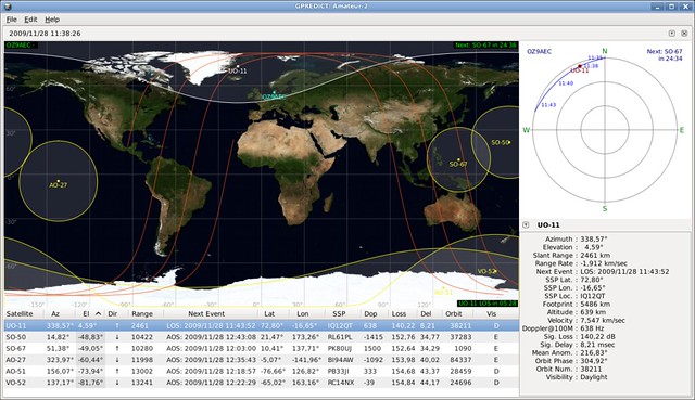
Gpredict (Linux/Windows/macOS, free, GPL) is the open-source standard. It propagates with SGP4/SDP4, draws the world-map ground track and the polar sky view, predicts passes, and — critically — drives both a rotator (via Hamlib rotctld) and a radio for full-Doppler tuning (via Hamlib rigctld) over TCP. It auto-updates TLEs from CelesTrak. For a Linux or cross-platform station it is the default recommendation.

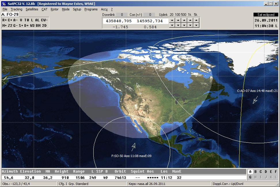
SatPC32 (Windows, paid/donationware, by DK1TB) is the long-standing Windows favorite, especially among linear-transponder operators. It is tightly integrated with rotator interfaces and CAT control, handles full-Doppler tuning elegantly with its “SatPC32ISS”/Doppler.SQF frequency files, and speaks the Yaesu GS-232 rotator protocol natively as well as via Hamlib. AMSAT distributes it as a membership benefit.

Orbitron (Windows, free) is a beautifully presented, widely used predictor and visualizer; it does rotator and radio control through a driver/DDE interface (often bridged to Hamlib or WiSP), and many operators use it purely for its clear pass predictions and sky views. Ham Radio Deluxe includes a satellite-tracking module integrated with its logging and rig-control suite — convenient for a station already living in HRD, commercial license. PstRotator is not a predictor at all but a universal rotator controller application: it takes az/el from Gpredict/SatPC32/Orbitron and translates to essentially every rotator-interface protocol in existence, making it the glue when your predictor and your controller box do not speak the same dialect.

On the web and mobile side, Heavens-Above and N2YO give browser-based pass predictions and live sky positions with no install (N2YO also has a real-time tracking API); Look4Sat (Android, open-source) and ISS Detector (Android/iOS) put pass prediction and a compass-guided sky pointer in your pocket — exactly what the Vol 33 “satellite in a backpack” handheld station wants. These do prediction, not station control.

Underneath all of them sits a programmatic layer worth knowing even if you only ever run a GUI. The Python sgp4 package is the reference SGP4/SDP4 implementation (Vallado’s code, wrapped); Skyfield builds on it to give clean observer-relative az/el/range/Doppler with proper time and frame handling in a few lines; the venerable predict (Linux, KD2BD) is a scriptable command-line/network predictor; and Hamlib provides rotctld and rigctld, the universal daemons that abstract every rotator and radio behind one network protocol (the next section). The SatNOGS project ties this layer into a global, open network of automated ground stations — its scheduler, client, and rotator/controller stack let stations worldwide observe and the SatNOGS DB aggregates the telemetry; it is both a way to receive birds you cannot see and the open-hardware reference for the DIY controller covered later.

Table 4 — Tracking software

Software	Platform	Rig (CAT) ctrl	Rotor ctrl	Full Doppler	Cost	License
Gpredict	Linux/Win/mac	yes (rigctld)	yes (rotctld)	yes	free	GPL (open)
SatPC32	Windows	yes	yes (GS-232 + Hamlib)	yes	~€40 donation	proprietary
Orbitron	Windows	via driver/DDE	via driver	via plugin	free	freeware
Ham Radio Deluxe	Windows	yes (HRD rig)	yes	yes	~$100	proprietary
PstRotator	Windows	(pass-through)	yes (all protocols)	(pass-through)	~€20	proprietary
Look4Sat	Android	no	no (predict only)	no	free	GPL (open)
Heavens-Above / N2YO	Web	no	no	no	free	web service

What to reach for. For a fixed automated station on Linux or cross-platform, Gpredict + Hamlib is the free, capable default. For a Windows linear-bird station, SatPC32 is the seasoned choice and its full-Doppler handling is excellent. If your predictor and controller box do not get along, PstRotator is the universal translator. For walk-and-track FM work, Look4Sat or a web predictor for the schedule and your own arm for the rotator. For scripting, automation, or building your own station logic, Skyfield (or raw sgp4) plus rotctld/rigctld.

34.8 Tracking via computer

The PC-driven station is the mainstream architecture and the one the other two control paths ultimately emulate. The principle: the tracking software, every second or so, propagates the current TLE to “now,” runs the frame transforms for your location, and produces a fresh (azimuth, elevation) for the rotator and a fresh Doppler-corrected (uplink, downlink) frequency for the radio. Those two outputs go out over two control channels, the antenna and the radio follow, and the loop repeats — a sampled closed loop running at ~1 Hz.

34.8.1 Rotator-control protocols

The az/el numbers reach the rotator’s controller box over one of a handful of serial/USB/TCP protocols. They differ in command syntax and in whether the controller reports its actual position back (closed-loop feedback) or merely accepts commands (open-loop). Knowing which your controller speaks, and which your software speaks, is the entire integration problem.

GS-232 (Yaesu) is the de-facto VHF/UHF amateur standard, an ASCII protocol over RS-232. Its core commands are human-readable: W aaa eee slews to azimuth aaa and elevation eee (e.g. W045 030), C queries azimuth, B queries elevation, C2 queries both, and single letters R/L/U/D jog the axes. The controller answers position queries with +0aaa+0eee-style strings, so it is a closed-loop protocol. GS-232A and GS-232B differ in minor framing details. Because Yaesu’s G-5500 + GS-232 combination has been the reference amateur az/el for decades, GS-232 is the protocol nearly every tracking program and nearly every third-party controller supports or emulates — it is the lingua franca.

EasyComm I / II / III is the open protocol that grew out of the WiSP/amateur-satellite world and is what the open-hardware controllers default to. EasyComm I is the simplest: an ASCII string like AZ180.0 EL45.0 sent to command position. EasyComm II adds position queries and finer control (AZ, EL, UP/DN for radio frequency, VE for version) and is the most widely implemented level. EasyComm III extends it further for advanced controller status. EasyComm is the protocol Gpredict speaks natively to a controller when not going through Hamlib, and it is what K3NG firmware and the SatNOGS controller expose, making it the natural choice for DIY.

SPID Rot2Prog is the binary protocol of the Alfa-SPID controllers (the MD-01/02 and the older Rot2Prog box). Unlike the ASCII protocols it uses fixed-length binary frames (a start byte, packed BCD position digits, a command byte, and an end byte) for set/stop/status, which makes it compact and robust but not human-typeable. It is closed-loop with high-resolution pulse feedback, and it is well supported by Hamlib and the major tracking programs.

Table 5 — Rotator-control protocols

Protocol	Format	Feedback?	Spoken by
GS-232A/B	ASCII (W aaa eee, C2)	yes (position query)	Yaesu controllers; emulated by RT-21, K3NG, most software
EasyComm I	ASCII (AZ… EL…), set-only	minimal	open controllers; simplest DIY
EasyComm II	ASCII + queries (AZ,EL,VE)	yes	Gpredict native; K3NG; SatNOGS
EasyComm III	ASCII, extended status	yes	advanced open controllers
SPID Rot2Prog	binary (BCD frames)	yes (pulse)	Alfa-SPID MD-01/02; Hamlib
Hamlib rotctld	TCP (P az el, p)	yes	the abstraction over all of the above

34.8.2 Hamlib as the universal abstraction

The way out of the protocol zoo is Hamlib, the Ham Radio Control Libraries. Hamlib provides two network daemons that turn every supported device into one uniform interface. rotctld is started with a backend driver for your specific controller (rotctld -m 603 … for GS-232B, -m 901 for SPID Rot2Prog, -m 204 for EasyComm II, and so on) and a serial port, and it then listens on TCP port 4533 for a tiny generic protocol: P 180.0 45.0 sets position, p gets it. rigctld does the identical job for radios over CAT, listening on port 4532, with F to set frequency and f to read it, abstracting Icom CI-V, Yaesu CAT, Kenwood, and the rest. The tracking software then only ever speaks “rotctld” and “rigctld” — it does not need to know whether the metal on the other end is a Yaesu, a SPID, or a homebrew Arduino. This is why Hamlib is the keystone of the modern tracked station: it decouples the software from the hardware, so any predictor that speaks Hamlib drives any controller that has a Hamlib backend, and a DIY controller becomes “supported everywhere” the moment it emulates a protocol Hamlib already knows (GS-232 or EasyComm).

34.8.3 CAT/Doppler correction, wiring, and the closed loop

The radio half of the loop is CAT (Computer Aided Transceiver) control. The tracking program computes the Doppler-corrected uplink and downlink frequencies each second and pushes them to the rig through rigctld, which continuously retunes the VFO(s). On a full-duplex satellite rig with two VFOs this corrects both links simultaneously (true full-Doppler); on a single-VFO rig the software corrects whichever link is active. The result is a downlink that holds a steady received pitch and an uplink that lands on the transponder’s nominal frequency despite ±10–55 kHz of drift.

Physically, the wiring is two control channels plus the RF. The rotator side runs from a USB-serial adapter (or a native serial port, or Ethernet for networked controllers) to the controller box, and a multi-conductor cable from the box up to the rotator’s motors and feedback sensors (Vol 33). The radio side runs from a USB-CAT cable (or the rig’s built-in USB) to the transceiver. Both can run over TCP, so the controlling PC need not be in the shack. Latency and update rate matter modestly: a 1 Hz update is ample for a LEO whose az/el changes a few degrees per second except in the keyhole, where a faster rate (4–10 Hz) and the flip-mode logic earn their place; serial latency of tens of milliseconds is negligible against a pass measured in minutes. The loop is “closed” in the sense that a feedback-reporting controller (GS-232 query, SPID status, EasyComm II) lets the software confirm the array actually reached the commanded angle and detect a stalled or lagging rotator — open-loop controllers slew on faith.

34.9 Tracking via a DIY controller

The DIY path builds the box that sits between the PC and the Vol 33 rotator — or replaces a commercial controller entirely. Its whole job is to take az/el commands in a standard protocol, drive the motors, read the position sensors, and report back. The unifying goal, stated in Vol 33, is to make a homebrew az/el rotator speak GS-232 or EasyComm so that the entire standard software stack above drives it with no special support.

34.9.1 The K3NG Arduino rotator controller

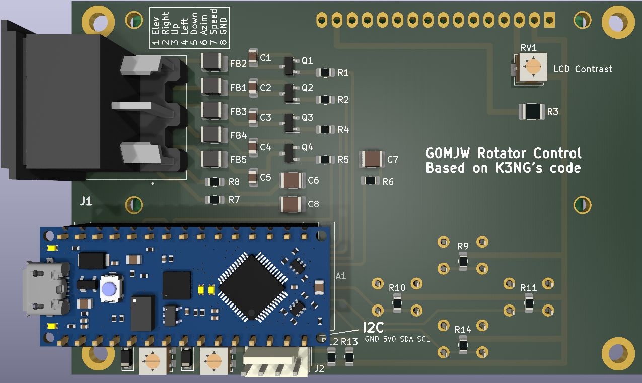
K3NG’s rotator controller is the canonical amateur DIY controller — open-source Arduino firmware (by Anthony Good, K3NG) that runs on an Arduino Uno/Nano/Mega and turns it into a full-featured az or az/el controller. Its decisive feature for satellite work is that it emulates both GS-232 (A and B) and EasyComm on its USB-serial port, so to Gpredict, SatPC32, or rotctld it looks exactly like a Yaesu GS-232 box — the “bridge from a homebrew az/el to standard software” in one firmware. It supports a wide range of position feedback (potentiometers, rotary/incremental encoders, the HMC5883/LSM303 compass, and absolute magnetic encoders), soft limits, calibration, speed ramping, and an optional LCD. K3NG is the recommended firmware whether you are driving relays into a surplus rotator’s motors or H-bridges into DC gearmotors: flash it, wire the feedback, calibrate the endpoints, and the homebrew rotator joins the standard stack.

34.9.2 The SatNOGS rotator controller stack

The SatNOGS controller is the open-hardware controller that pairs with the SatNOGS 3D-printed rotator from Vol 33. It is a microcontroller board (an STM32/Arduino-class design with stepper drivers) running the SatNOGS rotator firmware, which speaks EasyComm to the host. In a full SatNOGS station the SatNOGS client software schedules observations and commands the controller; standalone, the same controller takes EasyComm az/el straight from Gpredict. Because it is designed around stepper motors with the rotator’s known gear ratio, it can run effectively open-loop with micro-stepped position counting (homing once against an endstop on power-up), or closed-loop with an added encoder. It is the turnkey-ish DIY choice if you are building the SatNOGS mechanical design; the controller, firmware, BOM, and wiring are all published.

34.9.3 A homebrew Arduino/ESP32 + stepper-driver + AS5600 controller

The most instructive build is the from-scratch one, and it maps cleanly onto the Vol 33 “stepper + worm-gear + AS5600” rotator. The recipe: a microcontroller (an ESP32 is attractive for its Wi-Fi, so the controller can expose rotctld-style control over TCP, or a classic Arduino for simplicity), a stepper driver per axis (a DRV8825/A4988 for small NEMA-17 steppers, or a TB6600 for larger NEMA-23), an AS5600 12-bit absolute magnetic encoder per axis reading a diametric magnet on each output shaft over I²C, and firmware that closes the position loop and speaks GS-232 or EasyComm. The AS5600’s absolute nature is the key simplification: it knows its shaft angle at power-up, so no homing cycle is needed — unlike incremental encoders or bare step-counting, which must seek an endstop to establish a reference before they can be trusted. The worm-gear reduction from Vol 33 is self-locking, so the array holds against wind with the steppers idle.

Firmware, homing, and calibration. You can write the firmware from scratch (read both AS5600s over I²C, parse AZ…EL…/W… commands, run a simple proportional move-to-target on each axis with a deadband to avoid hunting, report position on query) — a few hundred lines — or, more pragmatically, run K3NG and configure it for the AS5600 and your stepper drivers, inheriting its mature GS-232/EasyComm emulation and calibration routines. Either way the bring-up sequence is: mount the magnets concentric with the shafts; verify each AS5600 reads a clean 0–4095 count over a full axis sweep (no skips, magnet centered); set the mechanical-to-electrical scale and the zero offset so that commanded 0° azimuth points true north and 0° elevation is the true horizon (a known star, the Sun’s computed az/el, or a compass-and-level for the coarse pass); set soft limits inside the mechanical stops; then point the box at a known high pass and confirm it tracks. An AS5600-absolute build needs this calibration only once.

Table 6 — A homebrew Arduino/ESP32 + stepper-driver + AS5600 controller

Part	Spec	Source	Mid-2026 price
Microcontroller	ESP32 dev board (or Arduino Uno/Nano)	Amazon / Mouser	$8
Stepper driver ×2	DRV8825 / A4988 (NEMA-17) or TB6600 (NEMA-23)	Amazon / Pololu	$6–24
Magnetic encoder ×2	AS5600 breakout + diametric magnet	Amazon / Mouser	$10
Stepper motors ×2	NEMA-17 (light array) / NEMA-23 (heavier)	(per Vol 33 rotator)	(in rotator BOM)
Logic + motor PSU	5 V logic + 12–24 V motor supply	Amazon	$15
USB-serial / Wi-Fi	(on the ESP32/Arduino)	—	$0
Enclosure, connectors, wiring	weatherproof box, terminal blocks, cable	hardware store	$20
Total (controller electronics)			~$60–80

The build cost is dominated by nothing — it is a weekend and ~$70 of parts on top of the Vol 33 rotator mechanics — and the payoff is a rotator that is indistinguishable, to the software, from an $800 commercial az/el.

34.10 Tracking via a COTS controller

The buy side replaces (or, for the Yaesu, is) the controller box: a commercial unit that bridges the PC to the rotator’s motors, speaks a standard protocol (or emulates GS-232), and brings polish — clean front-panel control, robust motor drive, calibration utilities, and known compatibility with the tracking programs. These pair with the Vol 33 commercial rotators (the G-5500, the Alfa-SPID RAS/BIG-RAS, the M2 OR-2800) and are dated mid-2026.

Yaesu GS-232B/A + G-5500. The reference amateur az/el control combination. The G-5500/G-5500DC rotator pair (Vol 33) is driven by Yaesu’s controller, and the GS-232B computer-interface unit (or the older GS-232A) adds the serial port and the GS-232 protocol that became the industry standard. Tracking software talks GS-232 directly or via Hamlib (rotctld -m 603). It uses the rotator’s potentiometer feedback, so it inherits the pot’s drift and needs occasional calibration, but it is the best-supported, most-documented satellite controller there is and the safe default. Roughly $700–800 for the rotator pair; the GS-232B interface is a few hundred more, and many newer G-5500 controllers include USB/serial.

Green Heron RT-21 (and RT-21az/el). A premium third-party controller (Green Heron Engineering) that drives a very wide range of rotators — including the Yaesu az/el and others — with high-precision digital position control, a calibration system, and GS-232 emulation plus its own protocol, so it integrates with all the standard tracking software. It is the upgrade path for an operator who wants better resolution and reliability than the stock Yaesu controller while keeping the G-5500 motors. Around $700–900 per axis-controller depending on configuration.

Alfa-SPID MD-01/MD-02 (Rot2Prog). The controller for the Alfa-SPID RAS/BIG-RAS rotators (Vol 33), speaking the binary Rot2Prog protocol with high-resolution pulse feedback. The MD-01 is the single/dual-axis controller; the MD-02 adds features. It is exceptionally repeatable (pulse feedback, no pot drift), supported by Hamlib (rotctld -m 901) and the major programs, and the natural controller for a medium-to-large CP-Yagi stack. The controller runs roughly $400–600; the RAS/BIG-RAS rotators it drives are $900–2200 (Vol 33).

M2 RC2800. M2 Antenna Systems’ controller for their OR-2800/MT-3000 az/el rotators and LEO packs — the big-station choice, with computer control and the precision to drive large arrays. The RC2800PX is the programmable, computer-controllable model that integrates with tracking software. It is the premium end, matched to M2’s heavy CP-Yagi arrays; budget $1500–2500+ for the M2 rotator-plus-controller system as a whole (Vol 33).

Which software drives which. In practice the matrix collapses because of GS-232 emulation and Hamlib: any controller that emulates GS-232 (RT-21, K3NG, and the Yaesu itself) or has a Hamlib backend (all of the above, plus SPID and EasyComm devices) is drivable by Gpredict, SatPC32, Orbitron (via driver/PstRotator), and Ham Radio Deluxe. The integration question is therefore almost always “what protocol does my controller emulate, and does my software (or Hamlib) have that backend?” — and for the four COTS units above the answer is yes across the board.

34.11 Worked examples

34.11.1 A full LEO FM-bird pass, end to end

The goal: work an FM “easy sat” — say SO-50 (a V/U FM bird, uplink 145.850 MHz, downlink 436.795 MHz, with a 67.0 Hz CTCSS tone required on the uplink) — from a fixed automated station with a Vol 33 crossed-Yagi LEO pack on a Yaesu G-5500, a full-duplex-capable rig, and a Linux PC running Gpredict and Hamlib. The sequence, concretely:

1. Refresh the elements. Let Gpredict auto-update from CelesTrak, or manually fetch the amateur.txt group: curl -O https://celestrak.org/NORAD/elements/gp.php?GROUP=amateur&FORMAT=tle. Confirm SO-50’s TLE epoch is within a couple of days. Confirm the PC clock is NTP-disciplined.
2. Predict and pick the pass. In Gpredict’s pass list, choose a pass with a comfortable max elevation (say 40–70°) — high enough for good signal, not so high it slams the keyhole. Note AOS time, max-el time and bearing, and LOS.
3. Start the control daemons. Rotator: rotctld -m 603 -r /dev/ttyUSB0 -s 9600 (GS-232B backend, serial to the GS-232/G-5500 controller, listening on :4533). Radio: rigctld -m <rig> -r /dev/ttyUSB1 (CAT backend, listening on :4532).
4. Wire Gpredict to both. In Gpredict’s Rotator Control point it at localhost:4533 and enable tracking; in Radio Control point it at localhost:4532, set the up/downlink frequencies and the V/U transponder, and enable full-Doppler (tune the 70 cm downlink — the higher band — actively; correct the uplink too). Choose flip vs non-flip for this pass per the keyhole.
5. Pre-position. A minute before AOS, command the rotator to the AOS azimuth and 0° elevation so the array is waiting where the bird will rise.
6. Acquire and work. At AOS Gpredict starts feeding P az el to rotctld and Doppler-corrected F freq to rigctld every second; the array tracks, the downlink holds a steady note. Key up with the 67.0 Hz tone, listen for your own downlink (full-duplex), and make contacts. Through TCA the azimuth will move fastest — if the pass is high, confirm the flip-mode behavior keeps you on the bird.
7. LOS and reset. At LOS Gpredict stops tracking; if you used flip-mode, let it return the array to a normal rest position for the next pass.

The same flow with SatPC32 on Windows differs only in the UI: SatPC32 talks GS-232 to the G-5500 controller directly (or via Hamlib) and drives the rig over CAT with its Doppler.SQF frequency file selecting the bird — the control loop and the operating steps are identical.

34.11.2 QO-100 — the geostationary “no-tracking” case

The contrast case ties back to Vol 33’s dish-and-LNB hardware. QO-100 (Es’hail-2) sits in a geostationary slot at 26° East: i = 0, e ≈ 0, period one sidereal day, so from your back yard it is motionless in the sky — a single fixed azimuth and elevation. There is no pass, no AOS/LOS, no rotator, and no satellite Doppler (range-rate ≈ 0). Tracking collapses to a one-time aiming calculation:

1. Compute the fixed look angle once. Treat the bird as a point at geostationary radius over 26° E and run the same topocentric transform from the “From orbit to your sky” section — or just use an online dish-pointing calculator or Gpredict with the QO-100 TLE — to get the azimuth, elevation, and (for an offset dish) the LNB skew for your latitude/longitude.
2. Aim and bolt down. Point the Vol 33 offset dish at that az/el, peak the received beacon by hand (small adjustments while watching the SDR waterfall), and lock the mount. Done — permanently.
3. Handle the only frequency instability, which is not Doppler. The 10.489 GHz downlink comes down through a TV-type LNB whose local oscillator drifts tens of kHz — invisible for wideband TV, fatal for narrowband SSB/CW. The fix is the Vol 33 hardware one: a reference-locked or Bullseye LNB so the narrow signals stay put. No tracking software, no rotctld, no rigctld Doppler loop — the geometry did all the work the instant you aimed.

QO-100 is the proof that “tracking” is a consequence of relative motion: remove the motion (geostationary) and the entire software-and-rotator apparatus of this volume reduces to one calculation and a wrench.

34.12 Regulatory note

Working a satellite uplink is transmitting, and it is governed by Vol 31 exactly as any other amateur transmission. The amateur-satellite service operates in segments of the 2 m, 70 cm, 23 cm, and 13 cm bands (and others), and your Amateur Extra authorization covers them, but the standard discipline applies: identify per the rules, observe the band-plan satellite sub-bands, run only the power you need (satellite work rewards less uplink power, not more — overdriving a linear transponder steals it from everyone else in the passband), and respect each bird’s published operating conventions (mode, the CTCSS tone an FM bird may require, the do-not-transmit-through-the-beacon etiquette on linear birds). Doppler-correcting your uplink so it lands on the satellite’s nominal receive frequency is part of being a good operator, not just a convenience — an un-corrected uplink drifts across the transponder and onto other QSOs.

The receive-only side — NOAA/Meteor weather at 137 MHz, GOES/Himawari L-band, Inmarsat/Iridium, GNSS — carries ordinary framing: receiving is unlicensed, but nothing here authorizes transmitting on those non-amateur allocations. The tracking software and controllers in this volume are agnostic to which case you are in; the regulatory line is drawn by what you key up, not by what computes the az/el.

34.13 Resources

• CelesTrak (celestrak.org) — Dr. T.S. Kelso’s TLE distribution (curated groups: amateur, weather, GOES, visual), plus his foundational columns on SGP4, TLE format, and coordinate systems — the single best free explanatory source for everything in this volume.
• Space-Track.org — the authoritative US Space Force (18 SDS) catalog and TLE source; free account required.
• AMSAT (amsat.org) — bird status and frequency lists, online and downloadable pass predictions, the satellite operating guides, and the SatPC32 distribution; the amateur-satellite community’s hub.
• Gpredict (gpredict.oz9aec.net) and SatPC32 (dk1tb, via AMSAT) — the two reference tracking programs; their documentation covers rotator and CAT setup in detail.
• Hamlib (hamlib.github.io) — rotctld/rigctld, the backend list (model numbers per controller and rig), and the protocol documentation — the universal control abstraction.
• SatNOGS (satnogs.org) — the open ground-station network: the open-hardware rotator controller, firmware, the client/scheduler stack, and the SatNOGS DB.
• K3NG rotator controller (github.com/k3ng/k3ng_rotator_controller) — the canonical open-source Arduino rotator-controller firmware with GS-232 + EasyComm emulation; the DIY-controller reference.
• python-sgp4 (Brandon Rhodes / Vallado) and Skyfield (rhodesmill.org/skyfield) — the reference SGP4 implementation and the high-level astronomy library for scripted prediction and az/el/Doppler.
• Vallado, Fundamentals of Astrodynamics and Applications — the standard modern text on the two-body problem, the frame transforms, and SGP4 (Vallado also maintains the corrected public SGP4 code). Bate, Mueller & White, Fundamentals of Astrodynamics is the classic, more compact companion.
• Hoots & Roehrich, Spacetrack Report No. 3 (1980) — the original SGP4/SDP4 definition; read alongside Vallado’s “Revisiting Spacetrack Report #3” (2006) for the corrected algorithms.
• Companion volumes: Vol 33 — Satellite Antennas & Rotators, the hardware this volume drives (the CP antennas, dishes/LNBs, and the G-5500/SPID/M2 rotators); Vol 29 (radio↔antenna use-case matrix); Vol 31 (regulatory & RF safety — the uplink-is-licensed-TX framing); Vol 3 (dB/dBm and link budgets — the slant-range path loss this volume’s range output feeds); Vol 28 (modeling software — the other “runs on a laptop” volume). Peer radios in the Hack Tools project: RTL-SDR (the canonical weather/QO-100-RX/L-band receiver), HackRF One (wideband RX and QO-100 uplink TX), Quansheng UV-K5 (the walk-and-track FM-bird HT).