Fan & Trap Dipoles — Parallel Resonators and LC Traps

---

2.1 About this volume

Vol 1 laid out the multi-band wire-antenna problem as a table of structural trades — off-center feed, parallel resonators, series LC traps, high-impedance tuner-fed doublets, compromise lengths, and switched links — and gave the off-center-fed dipole (OCFD) the full-depth treatment as the dive’s highest-utility, no-tuner default. This volume takes the next two rows of that table and develops each to the same depth: the fan dipole, which solves the multi-band problem by brute force — building a separate half-wave resonator for every band and paralleling them all on one feedpoint — and the trap dipole, which solves it by cleverness — inserting a frequency-selective network in each leg that switches a single wire between “insulator” and “loading coil” depending on which band you’re driving it on.

The two designs sit at opposite ends of an efficiency-versus-compactness axis, and understanding why is the point of this volume. The fan dipole pays for its multi-band coverage in mechanical complexity and antenna real estate — every band needs its own full-length wire, and the wires have to be kept far enough apart, and trimmed in the right order, that they behave as advertised. The trap dipole pays for its multi-band coverage in lost power — every trap between the feedpoint and a wire tip is a lossy component sitting in the current path on every band below its own design frequency, and no amount of clever winding makes that loss zero. Both facts are demonstrable rather than folklore, and this volume works through the mechanism behind each: the admittance argument that explains why a fan dipole’s inactive wires genuinely do stay out of the way, and the equivalent-circuit argument that explains exactly when and how much a trap costs you. Real trap-loss data (measured and published by Tom Rauch, W8JI, whose figures are the most frequently cited independent measurements in the amateur literature) is included in §6, and it complicates the folk wisdom about “roughly a dB per trap” more than it confirms it.

Scope stays inside the boundary Vol 1 set: these are still center-fed, multi-band wire dipoles. The remaining rows of Vol 1’s taxonomy table — the tuner-fed doublet, the G5RV/ZS6BKW compromise-length family, the linked dipole, and the wide-bandwidth cage dipole — get their own full treatment in this dive’s companion volumes; this volume does not duplicate them. Trap verticals (the Hustler-style multiband ground-mounted trap antenna) work on the same electrical principle developed in §5–§7 below but live in the hub’s Fixed Verticals dive, since the ground-image half of a trap vertical is a different structural problem than a symmetric trap dipole’s two legs.

2.2 Fan dipole — parallel resonators on a common feedpoint

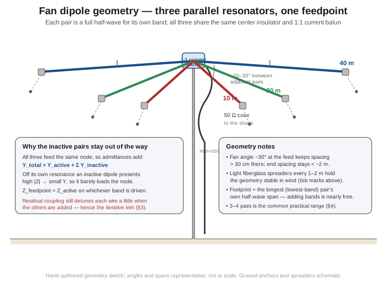
A fan dipole is the least clever and most honest of the multi-band solutions: build one ordinary half-wave dipole per band, cut and trimmed exactly as the Single-Band Dipoles dive’s reference dipole would be, and land all of them on the same center insulator and the same feedline. Mechanically the wires are strung outward from a common apex at a spread of angles — a “fan” — so that the mutual spacing between adjacent pairs stays large enough to keep interaction manageable while the whole assembly still hangs from a single support structure.

2.2.1 Why the inactive pairs don’t load the active one

The principle usually gets stated as “each band sees its own resonant pair; the others are high-Z off-resonance,” which is correct but worth deriving rather than just asserting, because the derivation is what tells you how much interaction to expect and why the trim procedure in §3 has to run in a particular order. All the fanned pairs land on the same two feedpoint terminals, so from the feedline’s point of view they are N two-terminal loads wired in parallel, and parallel loads combine by adding admittance, not impedance:

Y_total(f) = Y_active(f) + Σ Y_inactive,k(f).

At the frequency you’re actually driving, exactly one pair is at or near its own resonance — call it the active pair — and every other pair is being driven far from its resonance. A dipole driven well off its own resonant frequency presents a feedpoint impedance dominated by reactance, and the magnitude of that reactance is large (a single-band dipole driven at half its design frequency shows several hundred ohms of reactance, climbing to 1500 Ω or higher near a full-wave point — see the Single-Band Dipoles dive). Large |Z| means small |Y|, so every inactive pair’s contribution to the sum above is small compared to the active pair’s own admittance, and

Z_feedpoint(f) ≈ Z_active(f)

to good approximation. This is the entire justification for feeding a fan dipole with a plain 1:1 current balun and no matching network at all: on whatever band you key up, the feedpoint looks, to first order, like the single-band dipole the Single-Band Dipoles dive characterized in full — the same ≈70–73 Ω resonant resistance, the same balance requirement, the same choke.

“To good approximation” is doing real work in that sentence, though, and the residual is worth naming explicitly because it drives the whole of §3. Every inactive pair’s admittance is small but not zero, and it is reactive, so it adds a small parallel susceptance at the active pair’s feedpoint — physically, extra shunt capacitance from the neighboring wires sitting electrically short of their own resonance at the frequency in use. A small added shunt capacitance shifts a resonant load’s apparent resonant frequency down a little, which is exactly the “the parallel wires add capacitance, lowering the resonance” effect a builder observes on the bench: add the second and third wire to an already-trimmed single wire, and its resonance drifts down by tens to a couple of hundred kHz, not by nothing.

2.3 Fan dipole — mutual coupling, detuning, and the trim-order procedure

The practical consequence of §2’s admittance argument is that a fan dipole cannot be trimmed one wire at a time in isolation and then simply bolted together — each wire’s resonance shifts once its neighbors are physically present, because each neighbor’s small residual admittance is only there once the fan is assembled in its final geometry. The fix is an iterative sweep-and-trim procedure done with all the wires mounted in place from the start, not a sequence of independent single-band builds.

The order matters, and it matters for a reason grounded in §2’s math rather than superstition. Consider trimming the shortest (highest-band) wire last versus first. If you trim the shortest wire first, every wire you add after it (all lower in frequency, all longer) sits, relative to its own resonance, only slightly detuned by the one short wire already present — but the short wire itself is the element most disturbed by the process: each longer (lower-frequency) wire added afterward piles more shunt admittance onto the common feedpoint, and that loading keeps shifting the short wire’s effective tuning as the fan is built out. You end up chasing a moving target on the wire most sensitive to being last-trimmed. Trimming longest first avoids this: the lowest-band wire, once correctly resonated, is comparatively insensitive to whichever shorter wires get added afterward (their added susceptance is smaller in absolute terms relative to the long wire’s much larger reactance slope near resonance), so its trim tends to hold as the fan is built out. This is standard practice in the constructed-fan-dipole literature and is the same guidance a builder tuning a real 40/20/15/10 m fan will find repeated by hams who’ve built the same antenna: start with the lowest band, work up in frequency, and re-check the lower bands after each higher-band trim rather than assuming they’ll hold untouched.

The procedure, worked through in full:

1. Cut every wire 1–2% long. End-effect (the Single-Band Dipoles dive’s trim factor) already shortens the free-space half-wave a few percent; cutting long leaves margin for the coupling-driven downward shift §2 predicts, so you are always trimming (removing wire) rather than needing to splice more on.
2. Mount the full geometry before sweeping anything. All wires go on the center insulator and end-spacers in their final fan angle and spacing. Sweeping a single wire in isolation and expecting that number to hold once its neighbors are added is the single most common fan-dipole build mistake.
3. Sweep and trim the longest (lowest-band) wire to resonance first, exactly as a single-band build would proceed — NanoVNA at the feedline end, trim in small increments, re-sweep, converge.
4. Move to the next-shorter wire, sweep, and trim it to its own target, accepting that the just-trimmed longer wire is now a small parasitic load on it too.
5. Re-sweep every already-trimmed band after each new wire is trimmed. The longer wires will have drifted down slightly from the newly added shorter wire’s shunt capacitance; a few tens of kHz of drift per addition is typical and expected, not a sign of a bad build.
6. Iterate until every band lands within roughly 20–30 kHz of its target simultaneously. Three to five full passes through the wire set is a realistic expectation for a three- or four-band fan; this is, band-for-band, the most tuning-intensive build among the multi-band designs — the OCFD trims once, the fan dipole trims in a loop.

The reward for the extra bench time is that once converged, each band’s performance is essentially indistinguishable from an isolated single-band dipole — a claim §4 makes precise.

2.4 Fan dipole — feedpoint impedance, per-band pattern, and wire-count limits

2.4.1 Impedance and matching

With the trim procedure of §3 converged, each band’s feedpoint sits close to the ≈70–73 Ω resonant resistance the Single-Band Dipoles dive derived for the isolated element, modified by only the small residual coupling §2 quantified. That number is well inside the comfortable range for a 50 Ω feedline (the Single-Band Dipoles dive’s VSWR ≈ 1.46:1 mismatch-loss arithmetic applies unchanged), and the balance requirement is identical to a single-band dipole’s too — a fan dipole is still, per band, a symmetric two-terminal balanced load, so a 1:1 current balun at the shared feedpoint is the correct and sufficient choice. No impedance-transforming BALUN and no antenna tuner are needed on any band the fan was built for, which is the fan dipole’s principal selling point against the trap dipole (§9 makes the comparison explicit) and its shared advantage with a well-designed OCFD.

2.4.2 Pattern per band

Each active pair also radiates, to a good approximation, the pattern the reference half-wave already has — the free-space figure-8/donut and the ground-reflection lobing the pattern theory develops, unperturbed except for the (small) physical presence of the other, currently-inactive wires nearby. NEC modeling of representative fan-dipole geometries — this is a model-derived statement, not a bench measurement, and is presented as such — shows the inactive wires perturbing the active pattern by a few tenths of a dB at most, well below what a real installation’s ground clutter, height variance, and construction tolerance already contribute. The practical takeaway is that a fan dipole’s per-band pattern is worth treating as identical to a single-band dipole at the same height; the interaction that matters is the feedpoint detuning §2–§3 already covered, not the pattern.

2.4.3 Wire-count limits

Nothing in the physics caps the number of parallel resonators sharing a feedpoint — the admittance argument in §2 degrades gracefully as more wires are added, each contributing one more small parasitic susceptance term to the sum. What actually limits a real build is mechanical, not electrical, and it shows up in a specific order as the wire count climbs:

• Three or four pairs (six to eight wires) is the common practical ceiling for a residential single-mast fan dipole — enough to cover the busiest HF bands (80/40/20, or 40/20/15/10) without the feedpoint hardware becoming the weak point.
• The feedpoint terminal block is the first thing to run out of room. Every additional pair needs its own physical connection point, strain relief, and clearance from its neighbors at the one location where all the wires converge; a center insulator sized for three pairs is a tight fit for five.
• End-spacer discipline gets harder as bands multiply. Each additional wire needs its own run of fiberglass spreaders holding it at a stable fan angle in wind, and the spreaders themselves start interacting mechanically (and, at close spacing, electrically) once several wires share the same run.
• More bands than the mechanical ceiling is achievable, but fussy. Documented builds exist up to six parallel pairs (an 80/40/20/15/10/6 m fan dipole is a published amateur design), but the construction and tuning burden climbs faster than the band count — every added wire is one more sweep-and-trim pass in §3’s loop, and one more thing that has to survive wind loading at the shared feedpoint without shorting to a neighbor.

For most installations, the three-band 80/40/20 m fan is the best utility-per-effort point: it covers the three highest-traffic HF bands, needs no traps and no tuner, and the trim loop converges in a manageable handful of passes. Power handling is set purely by the wire gauge and the 1:1 balun rating — with no traps in the circuit, a fan dipole scales to legal-limit power exactly as a plain single-band dipole does, at whatever balun rating (Mix 31, sized for the band mix in use) you build or buy for it.

2.5 Trap dipole — the parallel-resonant LC trap and its equivalent circuit

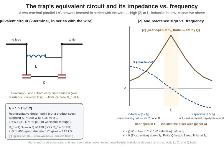
A trap dipole takes the opposite approach from the fan: instead of paralleling separate wires, it uses a single wire per leg, split into sections by inserting a two-terminal network — the trap — in series with the wire at one or more points. Each trap is a parallel-resonant LC tank: an inductor and a capacitor wired between the same two nodes, so that the wire on one side of the trap and the wire on the other side see the tank’s frequency-dependent impedance sitting between them rather than a plain conductor.

2.5.1 The parallel-tank impedance, derived

For an ideal (lossless) inductor L and capacitor C in parallel, the total admittance is the sum of each branch’s admittance:

Y(ω) = 1/(jωL) + jωC = j(ωC − 1/(ωL)).

The resonant frequency f₀ = 1/(2π√(LC)) is, by definition, the frequency at which the two branch admittances cancel: ωC = 1/(ωL), so Y(ω₀) = 0 and the ideal tank presents infinite impedance — a true open circuit — at exactly f₀. Away from resonance, the sign of the bracketed term tells you which branch dominates. Below f₀ (ω < ω₀), ωC < 1/(ωL), so the bracket is negative and Y is a negative-imaginary (inductive-type) susceptance — the same sign an inductor’s own admittance 1/(jωL) carries — whose reciprocal Z is therefore inductive (positive reactance). Above f₀ (ω > ω₀), the inequality flips, Y becomes positive-imaginary (capacitive-type), and Z is capacitive (negative reactance). This is the entire electrical basis for the trap dipole’s operation, and it maps directly onto the two panels of the geometry figure below:

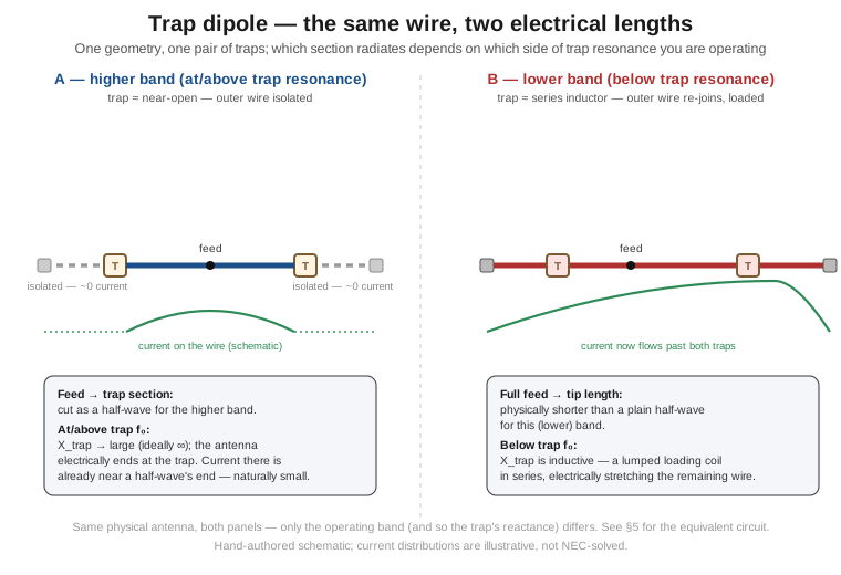
• At and above the trap’s own resonant frequency (panel A), the trap presents a very high impedance and the wire beyond it is, for practical purposes, electrically disconnected. The antenna behaves as if it physically ended at the trap, and the feed-to-trap section is cut to be a half-wave resonator for the higher band on its own.
• Below the trap’s resonant frequency (panel B), the trap’s reactance is inductive — it behaves as a lumped loading coil wired in series with the wire, exactly the mechanism a loaded mobile whip uses to appear electrically longer than it physically is. The wire beyond the trap is now electrically reconnected, and the loading inductance lets the total physical length (feed-to-tip) stay shorter than a plain half-wave at the lower band would otherwise require.

A real trap is not the ideal, lossless tank the derivation above assumes — every practical inductor has series resistance and every practical capacitor has some dielectric loss, and the combined effect is a finite Q, which turns the ideal open circuit at f₀ into a large but finite parallel resistance R_p = Q·X₀ (where X₀ = ωL = 1/(ωC) at resonance is the tank’s characteristic reactance). That finite R_p is where the trap’s power loss lives, and §6 works through how much it actually costs.

2.6 Trap dipole — Q, loss, and the bandwidth penalty

2.6.1 Trap Q varies enormously by construction

The single biggest determinant of how lossy a given trap is turns out to be how it’s built, not some fixed “traps lose X dB” constant. Measurements published by Tom Rauch (W8JI) — one of the most frequently cited independent sources on trap loss in the amateur literature, and the reference this section leans on — put a 40 m (7 MHz) coaxial-cable-wound trap at Q ≈ 134, while a discrete inductor paired with a high-quality air-variable or transmitting-grade capacitor at the same frequency measured Q ≈ 465 — better than a factor of three higher. Since R_p scales directly with Q, that difference alone is worth several times the loss resistance at resonance, before any question of trap placement or current is even considered. The ARRL’s own trap-antenna material makes the same point from the design side: a legal-limit trap build needs “quality high-voltage, high-current transmitting capacitors” precisely because ordinary components won’t hold the Q (or the voltage) a good trap needs.

2.6.2 Where the loss actually shows up

The naive mental model — “the trap dissipates power whenever it’s not at its own resonant frequency, because that’s when current flows through it” — is roughly right in spirit but glosses over a real subtlety that the same W8JI measurements bring out: the trap’s own loss resistance is largest, not smallest, exactly at its own resonance, because that is precisely where the reactive parts of Y cancel and the tank’s finite R_p is the entire remaining impedance rather than being partly masked by reactance. What saves a well-designed trap dipole from paying that peak-resistance penalty on its own band is current, not impedance: the trap sits, by design, at the electrical end of the higher-band half-wave (panel A of §5’s figure) — and the current at the end of a half-wave dipole is naturally near a minimum. Low current through a high (even if only finite-Q-limited) resistance is still low dissipated power. The real risk sits on the other, lower bands, where the same trap is now sitting well inside the current distribution (panel B), carrying substantial current while presenting a lossy inductive reactance rather than a near-ideal open circuit.

This is also why the ARRL’s design guidance is to resonate a trap off the exact middle of the band it’s meant to isolate — sometimes between two ham bands rather than centered on either — a placement that, done well, “can offer more bands with fewer traps, as well as greater efficiency” than centering the trap resonance squarely in the passband. The practical upshot for a builder: trap loss is not a fixed per-trap tax you can look up in a table. It is set by the trap’s Q (which is a direct function of how it’s wound and what capacitor sits in it), by exactly where its resonance is placed relative to the bands it’s meant to serve, and by how much current the antenna’s own current distribution happens to put through it on each band in use. Measured total losses in the W8JI data span from a few hundredths of a dB for a well-designed, well-placed trap pair up to around 1.6 dB combined for a more casually built coaxial-trap 40 m design — a real range, not a fixed number, and one that makes the folklore “expect about a dB per trap” both too pessimistic for a good build and, in the worst cases, not pessimistic enough.

2.6.3 The bandwidth penalty

Independent of the loss question, a trap-loaded section is narrower-bandwidth than the same physical wire length would be if it were a plain resonant half-wave, for the same reason any loaded-short antenna is narrowband: the trap’s own reactance changes quickly with frequency near its resonance (§5’s derivation shows X swinging from strongly inductive to strongly capacitive over a modest frequency span), and that fast reactance slope adds to the antenna’s own frequency sensitivity. The practical result, widely reported in the amateur trap-antenna literature, is a per-band 2:1-SWR bandwidth of roughly 1.5–2.5% for a trap-loaded band, against the 5–8% a clean, untrapped half-wave typically shows at the same frequency — a real and often underestimated cost on the lower bands of a multiband trap dipole, where the band itself (80 m in particular) is wide enough that a narrowed trap section can leave large stretches of the band outside a comfortable match.

2.7 Trap dipole — coax-cable traps, discrete LC, and power handling

2.7.1 The coax-cable trap

The most common homebrew and lower-cost commercial trap construction builds both the inductor and the capacitor from the same run of ordinary coaxial cable, wound into a coil. The winding — typically several turns of coax (commonly RG-58 or similar small cable) close-wound around a rigid PVC form for mechanical stability — supplies the inductance in the usual way any coil does. The capacitance comes from the coax itself: a length of coaxial cable is, intrinsically, a distributed capacitor between its center conductor and shield, with a per-foot capacitance set by the cable’s dielectric and geometry (common HF coax runs somewhere in the range of roughly 10–30 pF per foot depending on the specific cable). Terminating the winding by joining the center conductor at one end to the shield at the opposite end turns the whole coiled length into a single two-terminal parallel LC network — the coil supplies L, the cable’s own internal geometry supplies C, and the two are built from one continuous piece of hardware rather than as two separate discrete components. Because both L and C scale with the same physical winding, the design problem reduces to choosing a cable, a form diameter, and a turn count that land the resulting f₀ where you want it — a calculation every published coax-trap design works through, and one that has to be verified on the bench (a grid-dip meter or a NanoVNA in reflection mode across the unterminated trap) rather than trusted to the nominal numbers, because real cable capacitance-per-foot and real coil inductance both vary with the specific stock in hand.

2.7.2 Discrete L/C traps

The alternative is a discrete trap: a separately wound air-core coil (often larger-gauge wire on a rigid coil form, giving a higher, more controllable Q than a tightly wound coax coil) in parallel with a purpose-built capacitor — commonly a high-voltage silver-mica, doorknob ceramic, or (for adjustability during design) an air-variable capacitor. This is the higher-Q, and usually higher-cost and bulkier, route §6 already flagged (the ~465 vs. ~134 Q comparison), and it is the route legal-limit designs lean on specifically because a quality transmitting capacitor’s voltage and current ratings, not just its Q, matter once real power is flowing.

2.7.3 Power handling and voltage stress

A trap sees the same current as the rest of the wire it’s spliced into, but because it is a resonant (or near-resonant, off-band) reactive network, it can develop a voltage across its terminals substantially higher than a simple series-resistance calculation would suggest — the classic behavior of any high-Q reactive element carrying RF current. At legal-limit power (1.5 kW PEP) this voltage stress is the actual failure mode to design against: a trap capacitor that is under-rated for voltage arcs across its plates or through its dielectric, and a coax-trap’s winding can suffer insulation breakdown between turns or through the cable’s own dielectric if it’s pushed past its rating. This is precisely the concern behind the ARRL’s note that a legal-limit trap build needs genuinely rated “high-voltage, high-current transmitting capacitors” rather than whatever small-signal capacitor happens to be on hand — an underrated capacitor is both a Q problem (§6) and, separately, a reliability problem at power. The traditional trap-dipole failure signature that follows from a component running past its rating is audible and unambiguous on the air: a distinct “ping” as the trap arcs or opens, followed immediately by the SWR jumping toward infinity on whichever band that trap was serving — a clear diagnostic that the trap, not the rest of the antenna, has failed.

Weatherproofing matters here in a way it doesn’t for a plain wire splice, because a trap’s capacitance (whether from a discrete capacitor or the coax’s own dielectric) is part of the resonant circuit that sets f₀ — moisture ingress into a trap enclosure changes the effective dielectric constant around the capacitive element and detunes the trap, which shows up on the air as a resonance that drifts after rain even though nothing was touched. A sealed, weatherproof trap housing is accordingly not a cosmetic nicety on a trap dipole; it is protecting the electrical design point, not just the hardware.

2.8 The classic 80/40 and triband trap dipole — a worked example

The design procedure for a trap dipole runs from the highest band down, because the highest band’s half-wave section is a plain untrapped dipole and everything below it is built by adding trap-plus-wire increments. A two-trap, triband 80/40/20 m design illustrates the pattern cleanly:

• 20 m section (feed to first trap): cut as an ordinary 20 m half-wave dipole leg, exactly per the Single-Band Dipoles dive’s 468/f starting length, then trimmed to resonance with the traps already in place (the traps’ own end-to-end length and the small capacitive loading they add near their own resonance shift the raw formula length slightly, which is why the antenna is trimmed on the bench rather than built to the formula alone and trusted).
• First trap, resonant near 14 MHz: at and above 20 m, this trap presents a near-open and the antenna ends there — the 20 m half-wave the previous bullet describes.
• 40 m section (first trap to second trap): below the first trap’s resonance, that trap loads as an inductor, and the physical wire from the first trap out to the second trap is cut short of a full 40 m quarter-wave leg by an amount that depends on the trap’s inductive reactance at 40 m — a shorter physical run than an untrapped 40 m dipole would need, which is the entire point of building a trap antenna on a constrained lot.
• Second trap, resonant near 7.15 MHz: at and above 40 m, this second trap goes near-open and isolates everything beyond it — the feed-to-second-trap length now behaves as the 40 m half-wave.
• 80 m section (second trap to the tip): below both traps’ resonances, both load as series inductors, and the remaining wire out to the tip — again shorter than a full 80 m leg would otherwise need — completes the 80 m half-wave using the full physical length of the antenna.

A representative design calculation for the 40 m (second) trap illustrates the component values involved, worked from first principles rather than quoted from any particular product: targeting a characteristic reactance X₀ ≈ 250 Ω at f₀ = 7.15 MHz (a reactance level broadly consistent with the coaxial and discrete trap designs published in the amateur literature) gives

L = X₀/(2πf₀) ≈ 250/(2π × 7.15×10⁶) ≈ 5.6 µH,

C = 1/(2πf₀X₀) ≈ 1/(2π × 7.15×10⁶ × 250) ≈ 89 pF.

Those are realistic HF-trap-scale component values — a few microhenries and tens of picofarads is exactly the range published coax-trap and discrete-trap designs land in — but the exact L and C that land a specific winding or capacitor at exactly 7.15 MHz depend on the cable or coil and capacitor actually in hand, and belong on the bench (grid-dip meter or NanoVNA reflection sweep on the trap alone, before it ever goes on the antenna) rather than trusted to the formula in isolation. The physical shortening this loading buys — the amount of wire length a well-designed trap effectively “replaces” on the lower bands — is commonly on the order of several feet per trap in published multi-trap designs, enough that a five-band trap dipole (80/40/20/15/10 m) can come in a good deal shorter overall than an untrapped 80 m half-wave, which is precisely the real-estate case §9 weighs against the fan dipole’s honest, uncompromised, but longer footprint.

2.9 Fan vs. trap — choosing between the two

Both designs solve the same problem — more than one band on one feedpoint — by trading away something different, and the trade each makes points at a different installation constraint:

Table 1 — Both designs solve the same problem — more than one band on one feedpoint — by trading away something different, and the trade each makes points at a different installation constraint

	Fan dipole	Trap dipole
What you pay	Mechanical complexity — more wires, more spreaders, feedpoint crowding, an iterative trim loop	Real power loss on every band below each trap’s own resonance, plus narrower per-band bandwidth
Per-band efficiency	Essentially equal to a single-band dipole once trimmed	Reduced — by an amount that depends on trap Q and design, not a fixed number (§6)
Per-band bandwidth	Full single-band-dipole bandwidth (5–8%)	Narrowed by the loading traps (roughly 1.5–2.5%)
Physical footprint	Set by the longest (lowest) band’s own half-wave span	Shorter than an untrapped antenna for the same lowest band — the entire point of the loading
Matching	Plain 1:1 current balun, no tuner, on every band it was built for	Plain 1:1 current balun as well — the traps are a length/loss trade, not an impedance one
Failure mode	Mechanical — wire chafe, spreader failure, feedpoint corrosion	Electrical — trap capacitor voltage breakdown or winding arc-over, with a distinctive on-air “ping, then SWR to infinity” signature
Best fit	Enough real estate for the lowest band’s own half-wave span, and patience for the trim loop	A lot too small for the equivalent untrapped antenna, where the electrical shortening is worth the loss

The practical rule that falls out of this table is close to the one Vol 1 already reached from the taxonomy side: build the fan dipole if you have the real estate for it, because it is the only one of the two designs that doesn’t ask you to trade away power or bandwidth for its multi-band coverage — the cost is entirely up front, in build time and mechanical fuss, and none of it recurs every time you key the microphone. Reach for the trap dipole specifically when the lot genuinely cannot support the fan’s footprint — the loading is real and it does shorten the antenna, and for many residential and portable installations that shortening is the difference between “an 80 m antenna fits” and “it doesn’t.” What the trap dipole is not, despite decades of consumer marketing to the contrary, is a free multi-band upgrade with no downside; §6 and §7 above are the honest accounting of what a trap dipole actually costs, and a builder choosing between the two designs should weigh a real, if design-dependent, efficiency and bandwidth penalty against a real, and often decisive, reduction in required footprint.

2.10 Where this volume hands off

This volume took over the two multi-band solutions Vol 1’s taxonomy identified as feedpoint-shared parallel resonators and series-inserted frequency-selective networks, and developed each on its own terms. The fan dipole was shown to work by an admittance argument worth deriving rather than asserting — paralleled off-resonance dipoles present small admittance and so barely load the active resonator, Z_feedpoint ≈ Z_active — with the residual coupling that argument leaves over explaining both the observed on-bench detuning and the reason the trim procedure has to run longest-wire-first, converging over several passes to per-band performance essentially identical to a single-band dipole at the same height, with no matching network beyond the usual 1:1 current balun and no tuner on any covered band. The trap dipole was shown to work from the parallel-LC tank’s own admittance math — near-open at resonance, inductive below, capacitive above — mapped directly onto the physical picture of a wire that electrically ends at the trap on the higher band and re-extends, loaded, on the lower one; its real cost was quantified rather than assumed, using independently published (W8JI) Q and loss measurements that show trap loss is a strong function of construction quality and trap placement rather than a fixed per-trap tax, alongside the bandwidth-narrowing and voltage-stress consequences that come with any loaded, resonant, series-inserted network carrying real power.

The comparison table in §9 is this volume’s answer to “which one should I build,” and it hands off cleanly to the rest of the dive: this dive’s companion volume on the tuner-fed doublet and the G5RV/ZS6BKW compromise-length family covers the high-impedance, tuner-mandatory branch of Vol 1’s taxonomy that neither the fan nor the trap dipole represents, and the volume covering the linked and cage dipoles closes out the taxonomy’s remaining rows — switched-link band-change and brute-force bandwidth-widening — before the dive’s final volume works through a complete DIY build, a ranked commercial-buy survey, companion gear, and the cross-variant gotchas and myths that apply across every design this dive covers.

2.11 Resources

• ARRL Antenna Book (25th+ ed.), the multi-band and trap-antenna chapters — the canonical amateur reference for fan-dipole construction practice and trap design guidance, including the between-bands trap-resonance placement cited in §6.
• ARRL, “HF Trap Antennas” (arrl.org) — a curated collection of trap-antenna construction articles, including coaxial-cable trap designs and legal-limit trap-capacitor guidance cited in §6–§7.
• Balanis, Antenna Theory: Analysis and Design (4th ed.) — the mutual-impedance and parallel-element treatment underlying §2’s admittance derivation for the fan dipole.
• Tom Rauch (W8JI), trap-antenna measurements (w8ji.com) — the source for the trap Q and loss figures in §6; among the most frequently cited independent measured data in the amateur trap-antenna literature.
• K7MEM, “Multi-Band Coax Trap Antenna Design” — a widely referenced coaxial-cable trap construction and design-calculation reference, cited in §7 for the coax-trap construction method.
• Sevick, Transmission Line Transformers (5th ed.) — the current-balun theory behind the 1:1 balun both the fan and trap dipole feedpoints use unchanged.
• The Single-Band Dipoles dive, Vols 1–3 — the reference half-wave geometry, feedpoint impedance, and radiation-pattern theory this volume built on throughout without re-deriving.